The Colour Deconvolution 2 ImageJ plugin implements stain unmixing with Ruifrok and Johnston’s method described in [1]. The technique is useful to unmix dyes in images where colours mix subtractively (bright field microscopy using histological stains, watercolours or printed material using transparent inks). It is not suitable for fluorescence microscopy (fluorophores mix additively) or reflectance images. The code is based on a NIH Image macro kindly provided by A. C. Ruifrok with additional modifications. See the source code for the version history and contributors.
Installation: Download the jar file from this link and place it in the ImageJ/Plugins folder or folder under it. Restart ImageJ or execute Help>Refresh Menus. The new command should appear under the menu structure in Image>Color>Colour_Deconvolution2. The source code is included in the jar file.
Fiji users can alternatively use the Colour Deconvolution2 update site. This will uninstall the old version.
Any errors in old recorded macros failing to find the original plugin can be fixed by adding a “2” to the plugin call and including the desired output options. For example modifying the original call from:
run("Colour Deconvolution", "vectors=[H&E 2] hide");
to
run("Colour Deconvolution2", "vectors=[H&E 2] output=8bit_Transmittance simulated hide");
should produce the same output as the original plugin. However you might want to investigate the new features and options.
The MATLAB version is available from this link.
The plugin assumes images generated by colour subtraction (i.e. light-absorbing dyes such as those used in bright field histology, transparent inks on printed paper or watercolour paintings).
Brief description
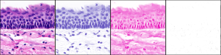
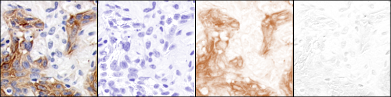
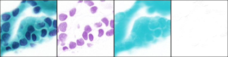
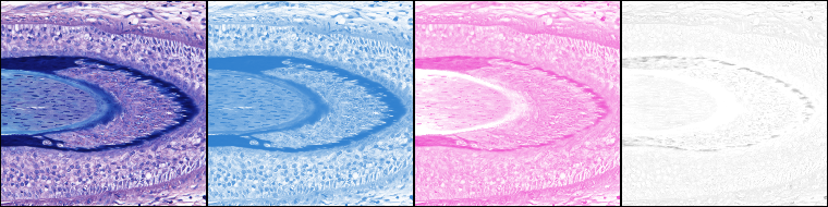
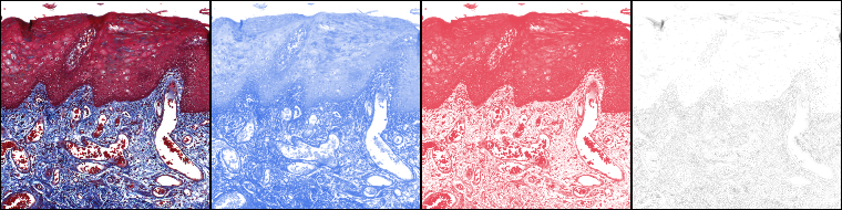
Input: The procedure expects a 24bit RGB image (or stack of images) generated by colour subtraction (typically bright field histology imges) already opened in ImageJ and unmixes the colour information into up to three dyes defined by the user.
Output: Four types of user defined outputs are supported:
- three 8bit transmittance images with or without colour look up tables,
- three 32bit transmittance images with or without colour look up tables,
- three 32bit absorbance images,
- one 24bit RGB intensity image where a particular dye has been removed or retained.
License:
Colour Deconvolution 2 plugin. Copyright (C) 2020 Gabriel Landini. This program is free software: you can redistribute it and/or modify it under the terms of the GNU General Public License as published by the Free Software Foundation, either version 3 of the License, or (at your option) any later version. This program is distributed in the hope that it will be useful, but WITHOUT ANY WARRANTY; without even the implied warranty of MERCHANTABILITY or FITNESS FOR A PARTICULAR PURPOSE. See the GNU General Public License for more details. You should have received a copy of the GNU General Public License along with this program. If not, see https://www.gnu.org/licenses/
Citation:
If the software is useful to you, please acknowledge it in your publications as follows:
Landini G, Martinelli G, Piccinini F. Colour Deconvolution – stain unmixing in histological imaging. Bioinformatics 2020, https://doi.org/10.1093/bioinformatics/btaa847
Please also cite the original technique described by Ruifrok and Johnston [1].
Usage
The plugin can be used interactively through the ImageJ GUI and it is macro-recordable. A public run method can be used to call the plugin from other programs without user interaction.
Input: A 24bit RGB image (or a stack of images) must be opened in ImageJ. Avoid using lossy-compressed file formats (like JPEG).
Vectors: This is a 3×3 matrix of values representing the absorbance (with values in the range 0 to 1) of the red, green and blue (RGB) components of up to three different dyes to be unmixed.
When the staining technique comprises of less than three dyes, the unused vectors should be set to 0, 0, 0. The plugin offers a set of “built in” stain vectors for testing which were determined experimentally, but users are strongly advised to determine their own vectors to achieve accurate stain separation (see below, Determining New Vectors). Using the built-in vectors ‘blindly’ is not a good idea because recipes for histological stains often vary, involving alternative chemicals or procedures that result in colour variations. The current built-in stain vectors are:
- Haematoxylin and Eosin (two different ones, H&E and H&E 2)
- Haematoxylin and DAB (H DAB)
- Haematoxylin, Eosin and DAB (H&E DAB)
- NBT/BCIP and Red Counterstain II
- Haematoxylin, DAB and New-Fuchsin
- Haematoxylin, HRP-Green and New-Fuchsin
- Feulgen and Light Green
- Giemsa
- Fast Red, Fast Blue and DAB
- Methyl Green and DAB
- Haematoxylin and AEC (H AEC)
- Azan-Mallory
- Masson Trichrome
- Alcian Blue & Haematoxylin
- Haematoxylin and Periodic Acid – Schiff (H PAS)
- Brilliant Blue stain (still experimental, might change)
- Astra Blue and Fuchsin
- RGB subtractive
- CMY subtractive
- User values entered by hand
- Values interactively determined from rectangular ROIs (useful to determine new vectors)
Output: Several types of output are available:
- 8bit Transmittance: Three 8bit images representing the transmittance of each of the dyes with the option of colour look up tables that correspond to the colour of the vectors (see the Simulated LUTs option).
Transmittance T is the ratio of light transmitted (I) through a material to the incident light I0:T = I/I0
Its value ranges from 0 to 1 and the images generated with this option are scaled to the 8-bit greyscale space (from 0 to 255).
- 32bit Transmittance: Three 32bit images representing the transmittance of each of the dyes with the option of colour look up tables that correspond to the colour of the vectors (see the Simulated LUTs option). Transmittance values are displayed in the range from 0 to 1 although occasionally some values can be outside this range.
- 32bit Absorbance: Three 32bit images representing the absorbance of each of the dyes.
Absorbance is defined as the logarithm in base 10 of the ratio of incident light to transmitted light through a material:A = log10(1/T)
This allows determining concentrations of a substance based on the Beer-Lambert law: the absorbance of light passing through a solution is directly proportional to the length of the path of light (l) through the solution and to the concentration (c) of the light absorbing substance:
A = εlc
where ε is the absorptivity (or molar attenuation coefficient) of the substance.
The displayed range of the absorbance images is from 0 and 2.41, but occasionally some values can be outside this range. This plugin treats pixel RGB components with value of 0 as having the minimum non-zero transmittance in the image (1/255, instead of 0) to avoid log10(0) in further calculations. - RGB outputs: These options generate an RGB intensity image with dyes removed or retained. Please note: 1) In two-dye staining methods (where the 3rd vector is determined programmatically) the third channel does not correspond to a given colour present in the original image. Consequently, retaining or removing the 3rd channel is likely to result in unexpected and incorrect results in the RGB intensity image. 2) Attempting to unmix images stained with 3 dyes using a two-dye vector will also lead to erroneous results.
More options:
Simulated LUTs: This option generates look up tables (LUTs) for each of the three transmittance images that simulate the saturation of the unmixed dyes. Note that those are not intensity values, but just a visualisation of the transmittance.
For two-dye staining methods with the 3rd vector determined using the cross product option, the 3rd channel has a greyscale LUT as it does not represent a given colour of the original image.
Unchecking this option generates greyscale images.
Cross product for Colour 3: When only two dyes are defined (and the 3rd dye vector is 0, 0, 0) this option computes the ‘missing’ vector as the orthogonal to the first two, using the crossed product which is equivalent to resolving the problem using the Moore-Penrose pseudoinverse [2]. Note that in that case the vector does not represent real colour information, but the residual of the deconvolution process.
When this option is unchecked, the procedure computes an alternative 3rd vector (following Ruifrok and Johnston’s code) that is a complementary of the other two vectors that can still be represented in the RGB cube.
This setting is ignored when three dyes are defined.
Show matrices: This option displays the following information in the ImageJ Log window:
- The determinant of the Computed Vector Matrix. If this value is zero, the matrix cannot be inverted and unmixing is not possible. The program will attempt to make the matrix invertible by adding a small value (0.001) to the rows, columns or diagonals of the Computed Vector Matrix containing all zeros. The determinant will be computed again (and reported as “first attempt”). If the determinant is still zero, a second attempt is made by adding 0.001 to all zero matrix coefficients. If the determinant still is zero, a warning will be shown in the Log window.
- The Input Vector Matrix holds the values stored in the built-in vectors, input via the User values vector option or obtained by sampling From ROI.
- The Computed Vector Matrix is the matrix obtained after the Input Vector Matrix is normalised to the vector lengths, after any attempts to make it invertible, if that was needed (see point 1).
- The Inverted Vector Matrix contains the values used internally for the unmixing step.
- A set of the Java statements describing the newly determined vectors, so they can be included in the source code as a new stain.
- A one-line macro example using the Input Vector Matrix. This is shown only when the values are determined from ROIs to facilitate further testing without having to retype all the numbers.
Hide Legend: Selecting this option hides the legend with the dye colours and the Computed Vector Matrix in float format. To see the double precision values used by the program, check the Show matrices option.
Suggestions and limitations
Please read the original paper [1] to understand how the procedure works and also consider these points before using the plugin:
- Background illumination correction is essential to provide both a neutral colour background and a uniformly illuminated field. The background of the image is expected to be as close to white as possible (for 24bit RGB intensity this is 255, 255, 255) in regions where there is no stain at all.
- Mixes of single colours (or mixes of grey dyes) cannot be unmixed with this method (most histological methods use dyes with significant differences in the stain matrix).
- Seriously consider determining your own staining vectors from single-dye stained sections. The plugin provides a number of built-in stain vectors determined experimentally, but you should determine your own vectors to achieve accurate stain separation. See the notes below on Determining New Vectors.
- Some histological dyes scatter light considerably, rather than absorbing it (e.g. silver impregnation methods) and therefore cannot be unmixed reliably.
- Staining intensity quantification is meaningful only when dye uptake is stoichiometric (e.g. Feulgen reaction for DNA). Immunohistochemical methods are unfortunately non-stoichiometric (like most histological dyes), making them unsuitable to measure ‘antigen expression’ based on DAB intensity. The main reasons are:
- Antigen-antibody reactions are non-stoichiometric, therefore “darkness of stain” does not equate to “amount of reaction products” or “expression” of a given antigen. In fact most histological stains are non-stoichiometric (one of the known exceptions is Feulgen stain, commonly used for DNA cytometry).
- Immunohistochemistry also uses a series of amplification steps to visualise the results, making it difficult to control what the final intensity of the amplified signal actually represents in terms of amount of antigen.
- The chromogen DAB does not follow Beer-Lambert law. See, e.g., the paper by CM van der Loos:
“The brown DAB reaction product is not a true absorber of light, but a scatterer of light, and has a very broad, featureless spectrum. This means that DAB does not follow the Beer-Lambert law, which describes the linear relationship between the concentration of a compound and its absorbance, or optical density. As a consequence, darkly stained DAB has a different spectral shape than lightly stained DAB.”
Further concerns have been raised in this message posted by Al Floyd to the ImageJ mailing list.
In resume, while colour deconvolution can be useful to segment immunostained structures (e.g. count cells, nuclei, identify structures) or for image enhancement (e.g. for colour blind observers), attempting to quantify DAB intensity as a measure of antigen expression using this plugin is not a good idea.
Examples
Ink/pigment separation (using ROI defined vectors).
The example below shows stain separation in an old manuscript using regions of interest (defined by the user) where stains were applied uniquely. The top part of the image was pasted from the same manuscript page to allow sampling the ink alone. (Image of MS408, folio 2 recto courtesy of the Beinecke Rare Book and Manuscript Library, Yale University).
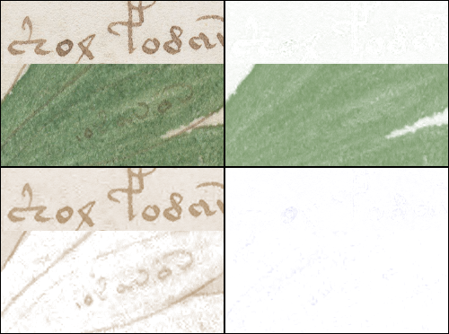
The vector values for this example were:
Colour[1] (green pigment):
   R1: 0.592132
   G1: 0.4580393
   B1: 0.6630081

 Colour[2] (brown ink):
   R2: 0.39982012
   G2: 0.55231196
   B2: 0.7315021

 Colour[3] (3rd component):
   R3: 0.69965965
   G3: 0.6965282
   B3: 0.15913807
Determining new vectors
1. Grab images of tissues stained with single dyes to ensure that the colour vectors are pure. For example, to create vectors for H&E, grab one image stained only with haematoxylin and one stained only with eosin. Apply background correction, so empty areas appear white. See this page for step by step instructions on background correction. Without background correction, the colours in the image will be affected by the colour/temperature of the light source and the unevenness background illumination of the light source optics, most likely preventing an accurate unmixing. Please read Haub & Meckel’s paper [3] reporting on the errors associated with dye unmixing using this technique, specially when using different types of brightfield illumination.
2. Stitch/paste these images together, so the single-stained regions all appear in the same collage image.
3. Run the Colour Deconvolution2 plugin and select the From ROI option to define example stained areas. Click OK on the plugin dialogue.
The plugin will then ask for rectangular selections of single dye regions. Select ROIs on areas which are all intensely stained (saturated) with only one dye, without empty background regions. Repeat this for other dyes.
If the staining method consists of only two dyes, when prompted for the 3rd selection just right-click. That vector will then be set to 0,0,0 and computed according to the option set for Cross product for Colour 3 as discussed above.
The deconvolution of the test image will take place and the stain separation can be evaluated. The Log window will show something like this (with different values, of course):
Matrix determinant: 0.46574739661107506

--- Input Vector Matrix --- From ROI
Ch3: cross product
Colour[1]: R1: 0.5389895695930097 G1: 0.7057613277058362 B1: 0.4597729789633545
Colour[2]: R2: 0.12477863655013832 G2: 0.7013660756270257 B2: 0.7017947846915321
Colour[3]: R3: 0.0 G3: 0.0 B3: 0.0

Note: When calling the exec() method of this plugin directly
from another plugin use the *Input Vector Matrix* above.

--- Computed Vector Matrix --- From ROI
C3: cross product
Colour[1]: R1: 0.5389895695930098 G1: 0.7057613277058363 B1: 0.45977297896335456
Colour[2]: R2: 0.12477863655013832 G2: 0.7013660756270257 B2: 0.7017947846915321
Colour[3]: R3: 0.37108194343891354 G3: -0.6889791029230941 B3: 0.6225801048771857

--- Inverted Vector Matrix --- From ROI
C3: cross product
Colour[1]: R1: 1.9757029514487046 G1: 0.392355764730999 B1: -0.743394728557563
Colour[2]: R2: -1.623555905020449 G2: 0.35416350878338454 B2: 1.3596379493260016
Colour[3]: R3: 0.37108194343891354 G3: -0.6889791029230941 B3: 0.6225801048771856

--- Java statements to include a new stain in the source code ---
if (myStain.equals("New_Stain")) {
// This is the New_Stain's Input Vector Matrix
MODx[0] = 0.5389895695930097;
MODy[0] = 0.7057613277058362;
MODz[0] = 0.4597729789633545;

MODx[1] = 0.12477863655013832;
MODy[1] = 0.7013660756270257;
MODz[1] = 0.7017947846915321;

MODx[2] = 0.0;
MODy[2] = 0.0;
MODz[2] = 0.0;

}

--- Macro example using the Input Vector Matrix determined from ROIs ---
run("Colour Deconvolution2", "vectors=[User values] output=[8bit_Transmittance] simulated cross [r1]=0.5389895695930097 [g1]=0.7057613277058362 [b1]=0.4597729789633545 [r2]=0.12477863655013832 [g2]=0.7013660756270257 [b2]=0.7017947846915321 [r3]=0.0 [g3]=0.0 [b3]=0.0");
4. Look in the Log window the text under the heading:
--- Java statements to include a new stain in the source code ---.
What follows are the Java statements that need to be included in the plugin’s source code, after line 191 where it reads “// Stains are defined after this line —–”. The source code should look like this (in red is the newly added code):
// Stains are defined after this line ------------------------
if (myStain.equals("New_Stain")) {
// This is the New_Stain's Input Vector Matrix
MODx[0] = 0.5389895695930097;
MODy[0] = 0.7057613277058362;
MODz[0] = 0.4597729789633545;

MODx[1] = 0.12477863655013832;
MODy[1] = 0.7013660756270257;
MODz[1] = 0.7017947846915321;

MODx[2] = 0.0;
MODy[2] = 0.0;
MODz[2] = 0.0;

}
5. Change the default name of the stain from “New_Stain” to the real staining method name (here it will be called “my new stain”).
6. When the 3rd colour is not defined (i.e. a staining method consists of only two dyes), just insert 0.0 values for the third component RGB values.
7. Add the real name of the stain in double quotes to the string array called “stain” (the order of names does not matter) so it matches the name given earlier. In the example below, note that the “New_Stain” name was appended at the end of the array (line 162) (in red is the newly added code):
String [] stain={"From ROI","H&E", "H&E 2","H DAB", "H&E DAB", "NBT/BCIP Red Counterstain II", "H DAB NewFuchsin", "H HRP-Green NewFuchsin", "Feulgen LightGreen", "Giemsa", "FastRed FastBlue DAB", "Methyl Green DAB", "H AEC","Azan-Mallory","Masson Trichrome","Alcian Blue & H","H PAS","Brilliant Blue","AstraBlue Fuchsin", "RGB","CMY", "User values","my new stain"};
8. Save the file and recompile the plugin from the ImageJ menu entry Plugins>Compile and Run…
9. Restart IJ or execute the Help>Update Menus command so the new class becomes active. The compiled version should now include the newly added stain vectors.
What is new
2.1 Release, 5/Aug/2022:
Added the plugin paper reference [4] (see the help button in the dialogue).
Added output for the Inverted Vector Matrix.
Output images preserve the spatial calibration of the original image (suggested by Jacqueline Ross).
2.0 Release, 21/Jun/2020:
Added an option for determining the 3rd undefined colour via cross product of the two other vectors. This is the correct way to determine it, yet the old method remains available (just uncheck the ‘Cross product’ option) for back-compatibility and historical reasons. Using the cross product for determining the 3rd colour can result in matrices with negative coeficients (i.e. ‘impossible’ colours), and therefore the LUT of the 3rd component determined this way will not represent a given colour in the image. Thanks to communications by Gloria Diaz, Mitko Veta and Peter Haub.
Pixels with intensity 0 are considered as having a value of 1 to avoid log(0) when computing absorbance. This convention is used in other programs (e.g. QuPath). Other alternatives are possible, like considering 0-intensity pixels as having a very small, but non-0 value, or even threat them as NaN (not a number) value. Please get in contact for instructions about the changes necessary to recompile the source code.
Added options to output LUTs images, 32bit images (transmittance, absorbance) and RGB (i.e. intensity) images. RGB output includes operations to remove or keep a particular colour. The same warning above remains for automatically determined 3rd vectors. Thanks to Filippo Piccinini for his help and testing.
Added an “RGB Retain all” option which is useful to understand how image colour data are processed by the colour deconvolution (e.g. dyes lacking “ideal”behaviour in terms of Beer-Lambert law).
Speeded up code > 3.2 times (Java 14) (thanks to Pete Bankhead and Peter Haub for their useful comments on pre-computing some formulae).
The code now checks whether the matrix can be inverted (non-zero determinant). If not, the program will attempt to make it invertible by adding a small value (0.001) to the rows, columns or diagonals that add up to 0. A warning is shown if “Show matrices” is checked. This is less drastic than the original code which added those small values to all 0 coefficients of the matrix. Be aware of any warnings when determining new vectors to be sure that the LUTs represent intended colours.
The option to show matrix values set in the dialogue is overridden and set to true when the input is via ROIs or User Values (because you will want to know what the results are).
The plugin now has a public exec() method that can be called directly without showing any images. The exec() method expects the *Input Vector Matrix* values.
An auto-generated macro is output to the log window when determining vectors from ROIs (this saves typing lots of numbers to apply the newly determined matrix).
Added a warning about determining your own vectors.
The Legend window now shows the Computed Vector Matrix which defines the colours shown (instead of the Input Vector Matrix which needs to be normalised, etc.).
References
[1] Ruifrok AC, Johnston DA. Quantification of histochemical staining by color deconvolution. Analytical and Quantitative Cytology and Histology 23: 291-299, 2001.
[2] Penrose R. A generalized inverse for matrices. Mathematical Proceedings of the Cambridge Philosophical Society 51(3): 406-413, 1955.
[3] Haub P & Meckel T. A Model based survey of colour deconvolution in diagnostic brightfield microscopy: error estimation and spectral consideration. Scientific Reports 5, 12096, 2015.
[4] Landini G, Martinelli G, Piccinini F. Colour Deconvolution – stain unmixing in histological imaging. Bioinformatics 2020, https://doi.org/10.1093/bioinformatics/btaa847
Acknowledgements
My thanks to Dr. A. Ruifrok for sharing his code for NIH-Image (the precursor of ImageJ) without which this plugin would not exist. Gloria Díaz, Mitko Veta and Peter Haub for their hints on the crossed product and its relation to the Moore-Penrose Pseudoinverse. Filippo Piccinini for various fixes, improvements and testing. Pete Bankhead and Peter Haub for their useful suggestions on code speed ups. Dennis Chao for incorporating the ability to process stacks. Wayne Rasband for creating and maintaining ImageJ.
Copyright © G. Landini, 2004-2023 (except where indicated).