Requires ImageJ 1.42m or newer.
These two plugins binarise 8-bit images (and 16bit images in the case of Auto_Threshold) using various global (histogram-derived) and local (adaptive) thresholding methods.
Latest version
Auto_Threshold v1.18, date: 12/Jan/2023
Auto_Local_Threshold v1.11, date: 8/Mar/2021
Installation
ImageJ: Copy the (Auto_Threshold.jar file) into the ImageJ/Plugins folder and either restart ImageJ or run the Help>Update Menus command. After this, two new commands should appear in Image>Adjust>Auto
Threshold and Image>Adjust>Auto Local Threshold.
Fiji: this plugin is part of the Fiji distribution, there is no need to download (it might show a different version number).
Auto Threshold
Use
Method selects the algorithm to be applied (detailed below).
The Ignore black and Ignore white options set the image histogram bins for [0] and [255] greylevels to 0
respectively. This may be useful if the digitised image has under- or over- exposed pixels.
White object on black background sets to white the pixels with values above the threshold value (otherwise, it sets to white the values less or equal to the threshold).
Set Threshold instead of Threshold (single images) sets the thresholding LUT, without changing the pixel data. This works only for single images. When processing a stack, two additional options are available: Stack can be used to process all the slices (the threshold of each slice will be computed separately). If this option is left unchecked, only the current slice will be processed.
Use stack histogram first computes the histogram of the whole stack, then computes the threshold based on that histogram and finally binarises all the slices with that single value. Selecting this option also selects the Stack option above automatically.
Note that the thresholded phase is always shown as white [255].
Since versions 1.8 and 1.1 of the two plugins respectively, the threshold of the binarised image is also silently set to 255 (i.e. not shown in red), so the particle analyzer should be able to pick the white pixels for the analysis.
Important notes:
1. This plugin is accessed through the Image>Auto Threshold menu entry, however the thresholding methods were also partially implemented in ImageJ’s thresholder applet accessible through the Image>Adjust>Threshold… menu entry. While the Auto Threshold plugin can use or ignore the extremes of the image histogram (Ignore black, Ignore white) the applet cannot: the ‘default’ method ignores the histogram extremes but the others methods do not. This means that applying the two commands to the same image can produce apparently different results. In essence, the Auto Threshold plugin, with the correct settings, can reproduce the results of the applet, but not the way round.
2. From version 1.12 the plugin supports thresholding of 16-bit images. Since the Auto Threshold plugin processes the full greyscale space, it can be slow when dealing with 16-bit images. Note that the ImageJ thresholder applet also processes 16-bit images, but in reality ImageJ first computes a histogram with 256 bins. Therefore, there might be differences in the results obtained on 16-bit images when using the applet and the true 16-bit results obtained with this plugin. Note that for speeding up, the histogram is bracketed to include only the range of bins that contain data (and avoid processing empty histogram bins at both extremes).
3. The result of 16 bit images and stacks (when processing all slices) is an 8 bit container showing the result in white [255] to comply with the concept of “binary image” (i.e. 8 bits with 0 and 255 values). However, for stacks where only 1 slice is thresholded, the result is still a 16 bit container with the thresholded phase shown as white [65535]. This is to keep the data untouched in the remaining slices. The “Try all” option retains the 16 bit format to show methods that might fail to obtain a threshold. Images and stacks that impossible to threshold remain unchanged.
4. The same image in 8 and 16 bits (without scaling) returns the same threshold value, however Li’s method originally would return different values when the image data was offset (e.g. when adding a fixed value to all pixels). The current implementation avoids this offset-dependent problem.
5. The same image scaled by a fixed value (e.g. when multiplying all pixels by a fixed value) returns a similar threshold result (within 2 greyscale levels of the original unscaled image) for all methods except Huang, Li and Triangle due to the way these algorithms work. E.g. the Triangle method applied to an 8 bit image and to the same
image converted to 16 bits with scaling can result in different threshold values. This is because the scaling from 8 to 16 bits creates empty bins in between the scaled grey values. The Triangle method (based on a geometric approach) finds those artefactual gaps in the new 16 bit histogram which satisfy the method constraints, but which would not exist in the original 8 bit image. This cannot be prevented (for example by detecting empty histogram bins) as it would interfere with the analysis when real empty bins (as oppose to artefactual ones) exist in the image.
6. Added bilevel image threshold. Thanks to Wayne Rasband and Wilhelm Burger. When the image consists of only 2 different pixel values (any two intensities) the plugin will automatically threshold it to values 0 and 255, while ignoring the selected thresholding method. This is because most methods expecting bi-modal histograms will fail as bilevel images can sometimes be interpreted as unimodal (e.g. an image consisting of two contiguous values in the histogram).
Try all
Which method segments your data best? You can attempt to answer this question using the Try all option. This produces a montage with the results from all the methods, so one can explore how the different algorithms perform on an image or stack. If you use stacks, you will realise that sometimes it might not be a good idea to segment each slice separately rather than with a single threshold for all slices (try the mri-stack.tif from the sample images to understand this issue).
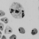
Original image
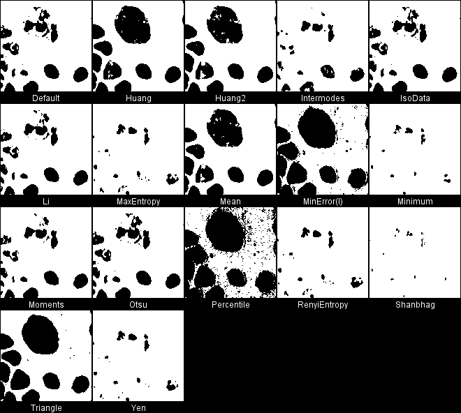
Try all methods.
When processing stacks with many slices, the montages can become very large (~13 times the original stack size) and one risks running out of ram. A popup window will appear (when stacks have more than 25 slices) to confirm whether the procedure should display the stack montages. Select No to compute the threshold values and display these in the log window.
Default
This is the original method of auto thresholding available in ImageJ which is a variation of the IsoData algorithm (see below). In this plugin the Default option should return the same values as the Image>Adjust>Threshold>Auto,
when selecting Ignore black and Ignore white.
While ImageJ tries to guess which pixels belong to the object and which to the background, this can be overridden and force segmentation of the desired phase with the White objects on black background option. The code in ImageJ that implements this function is the getAutoThreshold() method in the ImageProcessor class. The IsoData method is also known as iterative intermeans.
Huang
Implements Huang’s fuzzy thresholding method. This uses Shannon’s entropy function (one can also use Yager’s entropy function)
- Huang L-K, Wang M-J J. (1995) Image Thresholding by Minimizing the Measures of Fuzziness, Pattern Recognition, 28(1): 41-51.
Ported from ME Celebi’s fourier_0.8 routines http://sourceforge.net/projects/fourier-ipal
Huang2
This is a re-implementation of Huang’s fuzzy thresholding method by Johannes Schindelin to process more efficiently 16bit images and speed it up considerably. However on some images it does not return exactly the same result as the original method.
Intermodes
This assumes a bimodal histogram. The histogram is iteratively smoothed using a running average of size 3, until there are only two local maxima: j and k. The threshold t is then computed as (j+k)/2. Images with histograms having extremely unequal peaks or a broad and flat valley are unsuitable for this method.
- Prewitt JMS, Mendelsohn ML. (1966) The analysis of cell images, in Annals of the New York Academy of Sciences, vol. 128, pp. 1035-1053.
Ported from Antti Niemistö’s Matlab code. See http://www.cs.tut.fi/~ant/histthresh/ for an excellent slide presentation and the original Matlab code.
IsoData
Iterative procedure based on the isodata algorithm of:
- Ridler TW, Calvard S. (1978) Picture thresholding using an iterative selection method, IEEE Trans. System, Man and Cybernetics, SMC-8: 630-632.
This should return the same values as the Image>Adjust>Threshold>Auto, but it was implemented here to
allow pre-selecting the bright or dark phases in the image. (ImageJ tries to guess which is the object and which is the background).
The procedure divides the image into objects and background by taking an initial threshold,then the averages of the pixels at or below the threshold and pixels above are computed. The averages of those two values are computed, the threshold is incremented and the process is repeated until the threshold is larger than the composite average. That
is, threshold = (average background + average objects)/2.
A description of the method, posted to sci.image.processing on 1996/06/24 by Tim Morris:
Subject: Re: Thresholding method?
The algorithm implemented in NIH Image sets the threshold as that grey value, G, for which the average of the averages of the grey values below and above G is equal to G. It does this by initialising G to the lowest sensible value and iterating:

L = the average grey value of pixels with intensities <=G

H = the average grey value of pixels with intensities > G

is G = (L + H)/2?
yes: exit
no: increment G and repeat
Li
Implements Li’s Minimum Cross Entropy thresholding method based on the iterative version (Ref. 2) of the algorithm.
- Li CH, Lee CK. (1993) Minimum Cross Entropy Thresholding, Pattern Recognition, 26(4): 617-625.
- Li CH, Tam PKS. (1998) An Iterative Algorithm for Minimum Cross Entropy Thresholding, Pattern Recognition Letters, 18(8): 771-776.
- Sezgin M, Sankur B. (2004) Survey over Image Thresholding Techniques and Quantitative Performance Evaluation, Journal of Electronic Imaging, 13(1): 146-165. http://citeseer.ist.psu.edu/sezgin04survey.html
Ported from ME Celebi’s fourier_0.8 routines http://sourceforge.net/projects/fourier-ipal
MaxEntropy
Implements Kapur-Sahoo-Wong (Maximum Entropy) thresholding method:
- Kapur JN, Sahoo PK, Wong AKC. (1985) A New Method for Gray-Level Picture Thresholding Using the Entropy of the Histogram, Graphical Models and Image Processing, 29(3): 273-285.
Ported from ME Celebi’s fourier_0.8 routines http://sourceforge.net/projects/fourier-ipal
Mean
Uses the mean of grey levels as the trhreshold. It is used by some other methods as a first guess threshold.
- Glasbey, CA (1993), “An analysis of histogram-based thresholding algorithms”, CVGIP: Graphical Models and Image Processing 55: 532-537.
MinError(I)
An iterative implementation of Kittler and Illingworth’s Minimum Error thresholding. This version seems to be converge more often than the original implementation. Nevertheless, sometimes the algorithm does not converge to a solution. In that case a warning is reported to the log window and the result defaults to the initial estimate of the threshold which is computed using the Mean method.
- Kittler, J & Illingworth, J (1986), “Minimum error thresholding”, Pattern Recognition 19: 41-47
Ported from Antti Niemistö’s Matlab code See http://www.cs.tut.fi/~ant/histthresh/ for an excellent slide presentation and the original Matlab code.
Minimum
Similarly to the Intermodes method, this assumes a bimodal histogram. The histogram is iteratively smoothed using a running average of size 3, until there are only two local maxima. Threshold t is such that yt-1 > yt <= yt+1. Images with histograms having extremely unequal peaks or a broad and flat valley are unsuitable for this method.
- Prewitt JMS, Mendelsohn ML. (1966) The analysis of cell images, in Annals of the New York Academy of Sciences, vol. 128, pp. 1035-1053.
Ported from Antti Niemistö’s Matlab code See http://www.cs.tut.fi/~ant/histthresh/ for an excellent slide presentation and the original Matlab code.
Moments
Tsai’s method attempts to preserve the moments of the original image in the thresholded result.
- Tsai W. (1985) Moment-preserving thresholding: a new approach, Computer Vision, Graphics, and Image Processing, vol. 29, pp. 377-393.
Ported from ME Celebi’s fourier_0.8 routines http://sourceforge.net/projects/fourier-ipal
Otsu
Otsu’s threshold clustering algorithm. It searches for the threshold that minimizes the intra-class variance, defined as a weighted sum of variances of the two classes
- Otsu N. (1979) A threshold selection method from gray-level histograms, IEEE Trans. Sys., Man., Cyber. 9: 62-66.
doi:10.1109/TSMC.1979.4310076.
Wikipedia article on Otsu’s method: http://en.wikipedia.org/wiki/Otsu’s_method
Ported from ME Celebi’s fourier_0.8 routines http://sourceforge.net/projects/fourier-ipal
Percentile
Assumes a fraction of foreground pixels to be 0.5.
- Doyle W. (1962) Operation useful for similarity-invariant pattern recognition, Journal of the Association for Computing Machinery, vol. 9,pp. 259-267.
Ported from Antti Niemistö’s Matlab code. See http://www.cs.tut.fi/~ant/histthresh/ for an excellent slide presentation and the original Matlab code.
RenyiEntropy
Similar to the MaxEntropy method, but using Renyi’s entropy instead.
- Kapur JN, Sahoo PK, Wong AKC. (1985) A New Method for Gray-Level Picture Thresholding Using the Entropy of the Histogram, Graphical Models and Image Processing, 29(3): 273-285.
Ported from ME Celebi’s fourier_0.8 routines http://sourceforge.net/projects/fourier-ipal
Shanbhag
- Shanhbag A.G. (1994) “Utilization of Information Measure as a Means of Image Thresholding” Graphical Models and Image Processing, 56(5): 414-419.
Ported from ME Celebi’s fourier_0.8 routines http://sourceforge.net/projects/fourier-ipal
Triangle
This is an implementation of the Triangle method:
- Zack, G. W., Rogers, W. E. and Latt, S. A., 1977, Automatic Measurement of Sister Chromatid Exchange Frequency, Journal of Histochemistry and Cytochemistry 25 (7), pp. 741-753.
Incorporated from Johannes Schindelin’s plugin Triangle_Algorithm:
http://wbgn013.biozentrum.uni-wuerzburg.de/ImageJ/triangle-algorithm.html
http://www.ph.tn.tudelft.nl/Courses/FIP/noframes/fip-Segmenta.html#Heading118
The Triangle algorithm, being a geometric method, cannot tell whether the data is skewed to one side or another, but assumes a maximum peak towards one end of the histogram and one end towards the other. This causes a problem in the absence of information of the type of image to be processed, or when the maximum is not towards one of the histogram extremes (resulting in two possible threshold regions between that max and the extremes). Here the algorithm was extended to to find out to which side of the max peak the data goes the furthest, and search for the threshold within the largest range.
Yen
Implements Yen’s thresholding method from:
- Yen JC, Chang FJ, Chang S. (1995) A New Criterion for Automatic Multilevel Thresholding, IEEE Trans. on Image Processing, 4(3): 370-378
- Sezgin M. and Sankur B. (2004) “Survey over Image Thresholding Techniques and Quantitative Performance Evaluation” Journal of Electronic Imaging, 13(1): 146-165 http://citeseer.ist.psu.edu/sezgin04survey.html
Ported from ME Celebi’s fourier_0.8 routines http://sourceforge.net/projects/fourier-ipal
Auto Local Threshold
Use
Method selects the algorithm to be applied (detailed below).
The radius sets the radius (in pixel units) of the local domain over which the threshold will be computed,
White object on black background sets to white the pixels with values above the threshold value (otherwise, it sets to white the values less or equal to the threshold).
Special parameters 1 and 2 set specific values for each method. Those are detailed below for each method. It you are processing a stack, one additional options is available: Stack can be used to process all the slices.
Try all
Which method segments your data best? You can attempt to answer this question using the Try all option. This produces a montage with results from all the methods, so one can explore how the different algorithms perform on an image or stack. The Bernsen, Contrast and Midgrey mehtods can return similar results as they are based on the same basic idea of how to decide if a pixel is object or background.
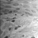
Original image
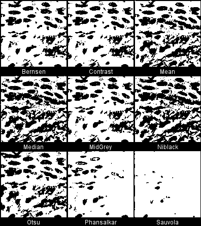
Try all methods.
When processing stacks with many slices, the montages can become very large (several times the original stack size) and one risks running out of ram. A popup window will appear (when stacks have more than 25 slices) to confirm whether the procedure should display the stack montages.
Bernsen
Implements Bernsen’s thresholding method. Note that this implementation uses circular windows instead of rectangular in the original.
Parameter 1: is the contrast threshold. The default value is 15. Any number different than 0 will change the value.
Parameter 2: not used, ignored. The method uses a user-provided contrast threshold. If the local contrast (max-min within the radius of the pixel) is above or equal to the contrast threshold, the threshold is set at the local midgrey value (the mean of the minimum and maximum grey values in the local window).
If the local contrast is below the contrast threshold, the neighbourhood is considered to consist only of one class and the pixel is set to object or background depending on the value of the midgrey.
if ( local_contrast <= contrast_threshold )
 pixel = ( mid_gray >= 128 ) ? object :  background
else
 pixel = (pixel >= mid_gray ) ? object : background
- Bernsen, J (1986), “Dynamic Thresholding of Grey-Level Images”, Proc. of the 8th Int. Conf. on Pattern Recognition
- Sezgin, M and Sankur, B (2004), “Survey over Image Thresholding Techniques and Quantitative Performance Evaluation”, Journal of Electronic Imaging 13(1): 146-165
Based on ME Celebi’s fourier_0.8 routines. http://sourceforge.net/projects/fourier-ipal
Contrast
Based on a simple contrast toggle. Sets the pixel value to either white (255) or black (0) depending on whether its current value is closest to the local maximum or minimum respectively.
The procedure is an extreme case of Toggle Contrast Enhancement, see for example:
- Soille P, Morphological Image Analysis: Principles and applications. Springer, 2004, p. 259.
This procedure does not have user-provided parameters other than the kernel radius.
Mean
This selects the threshold as the mean of the local greyscale distribution. A variation of this method uses the mean – C, where C is a constant.
pixel = ( pixel > mean - c ) ? object : background
Parameter 1: is the C value. The default value is 0. Any other number will change its value.
Parameter 2: not used, ignored.
Reference: http://homepages.inf.ed.ac.uk/rbf/HIPR2/adpthrsh.htm
Median
This selects the threshold as the median of the local greyscale distribution. A variation of this method uses the median – C, where C is a constant.
pixel = ( pixel > median - c ) ? object : background
Parameter
1: is the C value. The default value is 0. Any other number will change its value.
Parameter 2: not used, ignored.
Reference: http://homepages.inf.ed.ac.uk/rbf/HIPR2/adpthrsh.htm
MidGrey
This selects the threshold as the mid-grey of the local greyscale distribution (i.e. (max + min)/2. A variation of this method uses the mid-grey – C, where C is a constant.
pixel = ( pixel > ( ( max + min ) / 2 ) - c ) ? object : background
Parameter 1: is the C value. The default value is 0. Any other number will change its value.
Parameter 2: not used, ignored.
Reference: http://homepages.inf.ed.ac.uk/rbf/HIPR2/adpthrsh.htm
Niblack
Implements Niblack’s thresholding method:
pixel = ( pixel > mean + k * standard_deviation - c) ? object : background
Parameter 1: is the k value. The default value is 0.2 for bright objects and -0.2 for dark objects. Any other number than 0 will change its value.
Parameter 2: is the C value. This is an offset with a default value of 0. Any other number than 0 will change its value. This parameter was added in version 1.3 and is not part of the original implementation of the algorithm. The original
algorithm is applied when c = 0.
- Niblack, W (1986), An introduction to Digital Image Processing” Prentice-Hall
Based on ME Celebi’s fourier_0.8 routines. http://sourceforge.net/projects/fourier-ipal
Otsu
Implements a local version of Otsu’s global threshold clustering. The algorithm searches for the threshold that minimizes the intra-class variance, defined as a weighted sum of variances of the two classes.
The local set is a circular ROI and the central pixel is tested against the Otsu threshold found for that region.
- Otsu N. (1979) A threshold selection method from gray-level histograms, IEEE Trans. Sys., Man., Cyber. 9: 62-66.
doi:10.1109/TSMC.1979.4310076.
Please see also the Wikipedia article on Otsu’s global threshold method: http://en.wikipedia.org/wiki/Otsu’s_method
Ported from C++ code by Jordan Bevik.
Phansalkar
This is a modification of Sauvola’s thresholding method to deal with low contrast images.
- Phansalskar N. et al. Adaptive local thresholding for detection of nuclei in diversity stained cytology images. International Conference on Communications and Signal Processing (ICCSP), 2011, 218-220.
In this method, the threshold t is computed as:
t = mean * (1 + p * exp(-q * mean) + k * ((stdev / r) - 1))
where mean and stdev are the local mean and standard deviation respectively.
Phansalkar recommends k = 0.25, r = 0.5, p = 2 and q = 10. In this plugin, k and r are the parameters 1 and 2 respectively, but the values of p and q are fixed.
Parameter 1: is the k value. The default value is 0.25. Any other number than 0 will change its value.
Parameter 2: is the r value. The default value is 0.5. This value is different from Sauvola’s because it uses the normalised intensity of the image. Any other number than 0 will change its value.
Implemented from Phansalkar’s paper description, although this version uses a circular rather than rectangular local window.
Sauvola
Implements Sauvla’s thresholding method, which is a variation of Niblack’s
pixel = (pixel > mean * (1 + k *( standard_deviation / r - 1))) ? object : background
Parameter 1: is the k value. The default value is 0.5. Any other number than 0 will change its value.
Parameter 2: is the r value. The default value is 128. Any other number than 0 will change its value
- Sauvola, J and Pietaksinen, M (2000), “Adaptive Document Image Binarization”, Pattern Recognition 33(2): 225-236
Based on ME Celebi’s fourier_0.8 routines. http://sourceforge.net/projects/fourier-ipal