Here are some ImageJ macros and plugins that I have written.
Please make sure that you have the latest version of the ImageJ ij.jar file
| Disclaimer: The software in these pages is experimental. Use these plugins at your own risk. Although I have made every effort to make sure that they run as intended, there may be bugs and unexpected behaviour in instances that I have not envisaged. Please send any comments, problems or improvements to If no specific copyright notice is included, then consider the plugin as free software: you can redistribute it and/or modify it under the terms of the GNU General Public license as published by the Free Software Foundation; either version 2 of the license, or (at your option) any later version. These programs are distributed in the hope that they will be useful, but WITHOUT ANY WARRANTY; without even the implied warranty of MERCHANTABILITY or FITNESS FOR A PARTICULAR PURPOSE. See the GNU General Public License for more details. You should have received a copy of the GNU General Public License along with the programs; if not, write to the Free Software Foundation, Inc., 59 Temple Place – Suite 330, Boston, MA 02111-1307, USA. |
Align_4 (java & class files) This plugin allows manual alignment (movements in the x and y directions) up to 4 images. Supports transparency of the active image and selection of fiducial points (an origin and a target) for easy alignment. The plugin may be useful to build mosaics of smaller images.
Align_RGB_planes (java & class files) This plugin allows to shift (move in the x and y directions) stretch and rotate the red green and blue planes in an RGB image. Includes a macro to resize images so they are not affected by the cropping due to the rotation. Thanks to Leon Espinosa for suggesting the modification to log the net movement of the planes.
1.7 Supports stacks of RGB images. A set of buttons to move across the stack will appear when dealing with stacks. To align 48bit RGB stacks use the Align_Slice plugin.
1.9 Does All Slices.
Align_Slice (java & class files) This plugin allows to manually shift (move in the x and y directions) stretch and rotate a particular slice in an image stack.
Anaglyph (java & class files) Creates colour or greyscale, red-cyan or red-green anaglyphs, stereo pairs (crossed view stereo pairs) and depth-map images from the depth data and focused image generated with the extended depth of field plugin. The Anaglyph plugin expects both the “Height-Map” and “Output” images to be open (they hold the “topographical map” data and the “on focus” data). For Height-Map images created using other programmes, they can be 8 or 32 bits, but they should not be re-scaled (i.e. depth plane pixel values should be contiguous in the grey scale and start a 0). Because it cannot be known in advance the acquisition direction of the Z sequence, it may be necessary to invert the view sides when checking the red-cyan anaglyph. The plugin has been tested with only a small number of slices (6~20), so please report any problems.
A recent update of the Extended Depth of Field plugin changed the name of the “Topology” image to “Height Map”. and version 1.6 of the Anaglyph plugin also expects the new file name.
Auto_Threshold and Auto_Local_Threshold (link to jar file, source included) These plugins binarise 8-bit images using various global (histogram-derived) and local (adaptive) thresholding methods.
Requires v1.42m or newer. Copy the jar file into the ImageJ/Plugins folder and either restart ImageJ or run the Help>Update Menus command. After this 2 new commands should appear: Image>Adjust>Auto Threshold andImage>Adjust>Auto Local Threshold. Details and examples can be found here (local link) or at the Auto_Threshold and Aulto_Local_Threshold at the Fiji website wiki (external links).
Blend (java & class files) Blends (linearly) two greyscale or RGB images with a chosen mix ratio.
Colour_Correct (java & class files) This plugin corrects the colours of an image by first subtracting the mean RGB values of a number of selected points considered to be ‘black’ and then subtracts the background by performing the ratio of the image and the mean RGB values of a number of points considered to be ‘white’ minus the ‘black’. It does not correct for uneven illumination. The procedure is:
image = [(original-black)/(white-black)]*255.
This is a simple and quick (although not the best) method to compensate the filament temperature colour of light transmitted images such as bright field microscopy when there is no original illumination source available to perform the correction.
See this page explaining uneven bright field illumination correction.
1.3 Bug fix, popup menu disabled during right click.
1.4 Simplified code and improved rounding.
1.5 Fixed bug when no white sample points are selected.
Colour_Deconvolution2. A plugin implementing stain separation using Ruifrok & Johnston’s colour deconvolution method described in [1]. See this page for downloads and full details.
Convex_Hull_Plus (java & class files) This plugin calculates the convex hull and the minimum bounding circle of a binary set (formed by white or black particles).
The Convex Hull is the smallest convex polygon that contains the set. The plugin uses the ‘wrapping around’ (Graham scan) algorithm.
The Minimum Bounding Circle is the smallest circle that contains the set. An algorithm was modified from Xavier Draye’s posting to the ImageJ mailing list. I implemented so it does the calculations based on the convex hull points rather than the whole set (as the points that define the Minimum Bounding Circle must be in the Convex Hull). This should be speed up the computation. Please see the source code for details.
The plugin can display any of the above as a selection or draw them on the image. The plugin also displays in the Log window: the number of points in the Convex Hull, the length of the Convex Hull, the centre coordinates and radius of the Minimal Bounding Circle (in pixel units).
1.1 returns these values in floating point format.
1.2 fixes a bug in the Minimal Bounding Circle routine.
Dichromacy (java & class files) This plugin simulates the three main types dichromatic vision due to lack of function or absence of retinal photosensitive pigments: protanopia (red), deuteranopia (green) and tritanopia (blue cones deficiency). More details and examples can be found here.
IsoPhotContour (java & class files) and IsoPhotContour2 (java & class files).These plugins take a greyscale image and creates a new image [called IsoPhot] with up to 8 contour lines in the grey scale range. Isophotcontour2 can be drawn in different selected colours and depth levels. There is an option to draw the contour lines on a white or on a black background. There is also an option to convert the image to 8 bit colour image, otherwise the result is an RGB image.
1.2 Can process stacks.
IJ_Robot (java & class files) This plugin calls the Robot Java class. The purpose of the plugin is to allow the macro language to control other programs via programmed clicking and key presses.
When running the plugin one must specify an ‘order’ to the robot and some parameters (not all orders require all the parameters):
-
- Move: moves the mouse to a particular position (x, y) on the screen.
- [Left|Middle|Right]_Click: Clicks the mouse at a given (x, y) position with the chosen button.
- Delay: this is the time in milliseconds that the button is down during a click.
- [Left|Middle|Right]_Down: presses the chosen button at the current position (this order does not read the x, y coordinates).
- [Left|Middle|Right]_Up: releases the chosen button at the current position (this order does not read the x, y coordinates).
- KeyPress: this order will emulate typing the entered string, but will first Click (at the current position), so the cursor is guaranteed to focus in an entry box (maybe this click is not required, please send feedback or suggestions). KeyPress currently supports the following key presses: 0-9 a-z A-Z space /.,-
To emulate the [enter] key, type the exclamation mark ‘!’. Other characters are converted to ‘.’
Note that in Mac OSX with an AZERTY keyboard, the typed string does not get interpreted correctly. Be also aware that some OS do not support certain key presses. - GetPixel: reports to the Log window the r,g,b values of the pixel at the specified position (requires x, y coordinates). It will also return the Width and Height of the screen, as well as the coordinates of the pixel.
- CaptureScreen: this is similar to the IJ function Plugins>Utilities>Capture Screen.
A handy way to find the target coordinates is to first grab the screen (which opens as an image in ImageJ) and check the coordinates with the mouse (reported in the status bar).
Important: This plugin should be used with care because it is really easy to click in unintended places with undesired results. You have been warned!
- It may be necessary to increase the delay time for clicking orders depending on what is needed to be done and the response time of the target program.
- It may be also necessary to slow down the macro calls to this plugin between orders by using the macro command: wait(time_in_milliseconds). For instance when grabbing an image with an external programme, this might take some time to complete, and so calling further commands, these might not be executed while the image is being grabbed.
The included demo (updated on 7/9/2020), seems to work fine in various platforms. Make sure that there are no open images in IJ and that do not attempt move the mouse while running the macro.
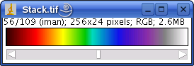
List_LUTs (java & class files) This plugin asks for a file (any file) in a folder where there are look up tables files (binary or text files as supported by ImageJ with a *.lut extension). The plugin then opens every LUT file in the selected directory and creates a new RGB stack (automatically saved as LUTs.tif in the “/plugins” folder) consisting of a LUT strip and (if selected) the name in each slice (the LUT name and the LUT values are also stored as metadata in each slice of the stack). If there are any corrupted LUT files in the folder, the plugin will exit.
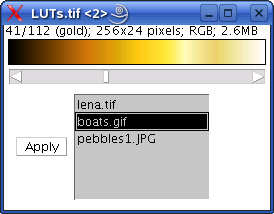
LUTs_ (java & class files) This plugin uses the RGB stack created with the plugin above (stored in “/plugins”) and creates a panel that allows browsing the different LUTs and apply any of them to any of the greyscale images currently open. Requires ImageJ 1.35l or better.
RCC8D and RCC8D_Multi. These are plugins implementing Discrete Mereotopology concepts and the Region Connection Calculus to perform spatial reasoning on image contents. More details and examples can be found here and in our page on Intelligent Microscopy.
Results_Histogram (java & class files) This plugin creates a histogram from a selected column of the Results Table data. Note that not everything that is shown in the Results window is necessarily in the Results Table. Incorporated into ImageJ 1.35g as the Analyze>Distribution… command.
Retinex (java & class files) This plugin is an implementation of the Retinex filter from the GIMP package. Retinex filtering is based on Land’s theory of image perception. Several algorithms exist and among these the multiscale retinex with colour restoration algorithm (MSRCR) combines colour constancy with local contrast enhancement so images are rendered in a similar way to the colour perception of the human vision. There appears to be a bug in the GMP filter, which was avoided here by using the built-in Gaussian filter of ImageJ. The Retinex plugin and examples are here.
The ImageJ plugin was written by Francisco Jiménez Hernández (UAEMex) jimenezf at fi.uaemex.mx during a research visit to Birmingham University School of Dentistry.
ThreePointCircularROI (java & class files) This plugin creates a circular ROI based on 3 user selected points on an image. The log window reports the coordinates of the centre of the circle and its radius. Co-linear points (that define an impossible circle) return a radius of -1.
Threshold_Colour ( jar file includes source ) This plugin (a modification of Bob Dougherty’s BandPass2 filter) allows to threshold a colour RGB images in the HSB, RGB, CIE Lab and YUV spaces. It supports extracting the range of HSB, RGB, CIE Lab or YUV values from a sample ROI (any type). Use: Extract the files from the zip archive and put them somewhere in the plugins directory (or subdirectory). The Threshold_Colour entry will appear in the Plugins hierarchy, depending on the subdirectory which the plugin is copied to.
1.7 Added a [Macro] button that generates a macro and sends it to the Recorder window (if active) based on the current plugin settings. The zip file also includes RGB2YUV and RGB2Lab plugins which are necessary for that macro (note that these plugins convert an RGB image to YUV and CIE Lab colour spaces but with values mapped into an 8-bit space).
1.8 added a warning and commented lines for back/foreground colours.
1.9 solved the problem of not applying the threshold if the original was being displayed.
1.10 added Select button. Fixed bug related to the name of files created with the image calculator command, solved bug in macro generated code for IJ v1.43h onwards.
1.11 background according to Binary>Options, thanks to Michael Schmid for several tips.
1.12 fixed the Selection button to return the proper ROI rather than the inverse of it, launch recorder if not active when pressing [Macro], added batch mode to the macro code. Version 1.15 the sRGB to Lab conversion now matches the colour space converter plugin in ImageJ.
1.16 fixed Lab space rescaling into 8 bits container.
Morphological Operators for ImageJ
Below is my collection of ImageJ plugins to perform various morphological operations.
All plugins are recordable. Some macros that make use of those plugins are also included.
Download the full Morphology set as a single zip file from here.
The zip file contains a Morphology folder with all the plugins and macros. Unzip the files in the plugins folder and finally restart ImageJ.
In Fiji, you can activate the “Morphology update site to install the collection.
Be aware that while most macros were written to deal with white regions, the plugins, deal with both, black or white regions (this means that the macros can be easily modified to deal with black regions too).
Please use this reference in your publications:
Landini G. Advanced shape analysis with ImageJ. Proceedings of the Second ImageJ User and Developer Conference, Luxembourg, 6-7 Nov, 2008. p116-121. ISBN 2-919941-06-2. Plugins available from https://blog.bham.ac.uk/intellimic/g-landini-software/
Add_Borders.class
This plugin set the pixels at the border of the image to black (0) or white (255) in the case of 8, 16 and 32 bits and to values (0,0,0) or (255,255,255) in 24bit images. This is used to set the image boundary values for special cases of binary and greyscale reconstruction, watershed transform and so on. Some of the macros in this collection use this plugin.
BinaryConditionalDilate_.class
This plugin dilates (3×3 neighbourhood, 8-connected) particles in an image (called seed) inside another image (called mask). The procedure can be applied n of times, or until idempotence if n = -1. In that case the procedure becomes is the same as BinaryReconstruction.
BinaryConditionalErode_.class
This plugin erodes (3×3 neighbourhood, 8-connected) particles in an image (called seed) except what is masked in another image (called mask) (i.e. the mask “protects” what should not be eroded). it can be applied n times, or, until idempotence if n = -1.
BinaryConnectivity_.class
Returns the number of connected pixels (+1) to each foreground pixel (8 neighbours): background=0, single pixel=1, end of a line=2, bifurcations=3, triple points=4, etc. To see the result, please adjust the Brightness/Contrast, or use high contrast or decorrelated LUT such as glasbey.lut (included in this collection).
BinaryDilate_.class
This plugin performs a 3×3 8-neighbour Binary Dilation of a binary image. The differences with the built in Dilation in ImageJ are:
- It checks that the image is binary [0] & [255]
- Processes all pixels in the image (ImageJ leaves the borders without processing).
- Supports “coefficients” (0-7). This is a logical constrain of the operation to locations where the number of neighbouring pixels in the opposite state is the coefficient: Classical dilation (0), Filling of single pixels holes (7), Filling of small crack lines (6), Filling of (some) irregular holes (5). See reference [2] for further details.
- can be applied n times without using SetIterations. Use -1 for dilation until the image is idempotent (no more changes).
- BinaryDilateTest.txt is a macro that shows the effect of the different coefficients.
Notice: This plugin will be discontinued since ImageJ 1.33q fixed a bug that prevented border processing and also implements the use “coefficients”. Note, however that in ImageJ, the coefficients range from 1 to 8 instead of 0 to 7.
BinaryDilateNoMerge4_.class
BinaryDilateNoMerge8_.class
These plugins perform a conditional binary dilation of a binary image (without merging particles together). The results are similar to a binary watershed transform of the background, partitioning it into areas of influence of the particles. Dilations are done with 4 or 8 pixel structuring elements respectively. The number of iterations can be set. Use -1 for dilation until idempotence.
Very slow, maybe there are better algorithms, but slow seems better than nothing…
To dilate without merging until idempotence, the macro Influence_Zones.txt described below is faster, although the principle underlying the algorithm is a different one.
BinaryGeodesicDilateNoMerge8_.class
This plugin performs a conditional binary dilation of a binary image (seed) inside another binary image (mask), without merging the seeds when they meet. The results are similar to a the BinaryDilateNoMerge8, but the operation is done inside a mask and so it restricts the dilation to the mask. The number of iterations can be set. Use -1 for dilation until idempotence.
Very slow, maybe there are better algorithms, but slow seems better than nothing…
BinaryErode_.class
This plugin performs a 3×3 8-neighbour Binary Erosion of a binary image.
The differences with the built in erosion in ImageJ are:
- Processes all pixels in the image (ImageJ leaves the borders without processing)
- Supports “coefficients” (0-7). This is a logical constrain of the operation to locations where the number of opposite state neighbours is the coefficient: Classical erosion (0), Removal of single pixels (7), Pruning of 8-connected lines (6), Removal of (some) irregular particles (5). See reference [2] for further details.
- Can be applied n times without using SetIterations. Use -1 for erosion until the image is idempotent (no more changes)
- BinaryErodeTest.txt is a macro that shows the effect of the different coefficients.
- BinaryPrune.txt is a macro that prunes all the branches of a binary skeleton, leaving only the closed loops. See also PruneAll.txt for another pruning method.
Notice: This plugin will be discontinued since ImageJ 1.33q fixed a bug that prevented border processing and also implements the use “coefficients”. Note, however that in ImageJ, the coefficients range from 1 to 8 instead of 0 to 7.
BinaryFill_.class
BinaryFill_2.class
These plugins fill holes in 8-connected particles (and also in child-particles) of a binary image. This function was incorporated in ImageJ v.1.31o (Process->Binary->Fill holes).
BinaryFill_2 is a much faster version, that uses ImageJ’s flood fill.
- Fill_Border_Holes.txt Fills holes including those touching the borders of the image This cannot be done with the “Fill Holes” command alone. Holes are assumed to be not only the traditional 4-connected background elements, but also those that touch the image borders, but extending no more than 2 contiguous borders (i.e. touching one border or a corner).
- Hole_Counter.txt Counts the number of particles, holes and Euler number of a binary image (with white particles on a black background). The Euler number is computed as the number of particles minus the number of holes and it is a measure of the topology of the image. (Works only for white particles on a black background). See the Euler.txt macro for a another method of computing the Euler number.
- FillHolesReconstruct.txt Fills holes of white particles on a black background, using the traditional method of reconstructing the inverse of the background using the (empty parts of) borders of the image as seeds.
BinaryFilterReconstruct_.class
This plugin filters 8-connected particles in a binary image that otherwise would disappear after n erosions. This technique is also called opening by reconstruction or inf-reconstruction. The difference with morphological Opening is that BinaryFilterReconstruct preserves the original shape or the particles (while opening tends to smooth the boundaries of particles). The algorithm is n erosions, followed by a Binary Reconstruction of the original image based on the eroded image as the seed.
The macro BinaryFilterReconstruct.txt shows how to implement this as a macro using the BinaryReconstruct plugin.
1.3 Changed ‘dilations in a mask’ for ‘floodfill8 in the mask from the seed’ to speed up.
1.4 Fixed bug with black particles and inverted LUTs.
1.5 Slight speed improvement.
1.6 Speed up by using 1D arrays.
BinaryHitOrMiss_.class
This plugin returns the locations of the image that match the kernel pattern.
The pattern is defined by a 3×3 square neighbourhood where 0=empty, 1=set, 2=don’t care.
- Corners.txt Returns the corners of a binary particle based on the Hit-or-miss transform.
- Euler.txt: Estimates the Euler number of a binary image using the hit-or-miss transform and a method described in ref. [4]. The result is accurate as far as the objects do not touch the border of the image. The Hole_Counter.txt macro does not have this issue.
BinaryLabel8_.class and BinaryLabel_.class
ImageJ plugin for labelling particles (8 neighbours) in a binary image.
BinaryLabel8_ can label up to 65530 particles in a unique greyscale value (from 1 to 65531), after that, the colours are recycled.
The output is a new 16 bit greyscale image with re-scaled brightness.
BinaryLabel_ can label more particles thant the above, as it stores the result in a 32bit image.
The BinaryLabelMacro.txt macro does a similar job.
One ideal look up table (LUT) that maximises the contrast between labelled particles is glasbey.lut (included in the zip file). Please read about it in Chris Glasbey’s website (reference: Glasbey, C.A., van der Heijden, G.W.A.M., Toh, V.F.K. and Gray, A.J. Colour displays for categorical images, Color Research and Application, 32, 304-309, 2007.).
BinaryReconstruct_.class
This is a very powerful morphological operation that reconstructs (retains) 8-connected particles in an image (called mask) based on markers present in another image (called seed).
Morphological Reconstruction consists of dilating the seeds inside the mask (so particles that do not have seeds are not reconstructed).
1.5 Changed ‘dilations in a mask’ for ‘floodfill8 in the mask from the seed’ to speed up.
2.0 Rewrite following the guidelines found here. Apart from being about 4 times faster, it can be called from another plugin without having to show the images. The plugin does not process stacks anymore, but that was not commonly used anyway and it can be achieved by a simple macro to process one slice at a time.
To call the binary reconstruction plugin from another without displaying the images use, for example:
   BinaryReconstruct_ br = new BinaryReconstruct_();
   Object[] result = br.exec(img1, img2, null, false, true);
   //parameters above are: mask ImagePlus, seed ImagePlus, name, create new image, white particle
   if (null != result) {
      String name = (String) result[0];
      ImagePlus recons = (ImagePlus) result[1];
   }
This procedure is called “Feature-AND” in reference [2].
2.1 Supports 4-neighbour connectivity.
2.2 Speed up by using 1D arrays.
- Hysteresis.txt: This macro uses Binary Reconstruction to aid thresholding an image.
Hysteresis thresholding (sometimes called double threshold) is useful to segment, for example, edge gradients. The macro assumes that the object is bright (usually the gradient after applying some edge detector).
First set the threshold of the “safe zone” (that surely belongs to the “object”) then set the threshold for the “unsafe zone” (which for sure is outside the “object”). The zone in-between is the “fuzzy zone”. Hysteresis thresholding adds parts of the fuzzy zone that are connected to the safe zone.
The macro creates 2 images: “Reconstructed” is the hysteresis-thresholded image, while “Result of Result” shows the safe zone (white), the pixels added to the safe zone (yellow), the pixels of the fuzzy zone not added (purple) and the unsafe zone (black).
The “Reconstructed” image corresponds to the white+yellow components of the “Result of Result” image.
A similar alternative to hysteresis thresholding is to perform n geodesic dilations of the safe zone masked by the fuzzy zone. This way one can control how far from the safe zone the fuzzy pixels that connected to it are to be added.
BinaryKillBorders_.class This plugin deletes binary objects that intersect the image border.
BinaryThick_.class
BinaryThick2_.class
These two plugins dilate the locations of the image that match one (BinaryThick_.class) or two (BinaryThick2_.class) kernel patterns.
First dilates then rotates the kernel, if set to do so. The pattern is a 3×3 neighbourhood where 0=empty, 1=set, 2=don’t care.
- ConvexHull1.txt: a morphological convex hull — square shape (not the true convex hull)
- ConvexHull2.txt: a morphological convex hull — diamond shape (not the true convex hull)
- ConvexHull3.txt: a morphological strong convex hull. If done with ‘rotate 90’ it gives a quasi-convex hull (not the true convex hull)
BinaryThin_.class
BinaryThin2_.class
These two plugins erode the locations of the image that match one (BinaryThick_.class) or two (BinaryThick2_.class) kernel patterns.
First erodes then rotates the kernel, if set to do so. The pattern is a 3×3 neighbourhood where 0=empty, 1=set, 2=don’t care.
- Boundary4.txt: produces a 4-connected boundary of particles
- Boundary8.txt: produces a 8-connected boundary of particles
- Diagonal8to4.txt: Converts 8 connected white features to 4 connected ones by filling empty diagonal pixel spaces
- H-break.txt: removes the centre of H-connected pixel patterns
- Influence_Zones.txt: creates influence zones by skeletonisation of the background followed by pruning. This is an alternative and fast way of “dilation without merging until idempotence”
- MCentroids.txt: creates the morphological centroids by thinning. The centroid of an object with a hole is a ring, otherwise it is a point.
- Prune1.txt: prunes a binary skeleton once.
- PruneAll.txt: prunes a binary skeleton until idempotence.
- Skeleton1.txt: an 8 connected skeleton, different from the one in ImageJ.
- Skeleton2.txt: an 8 connected skeleton, different from the one in ImageJ. It creates many lateral “bones” or branches.
- Skeleton3.txt: similar to skeleton1 but 4-connected.
- Skeleton4.txt>: this computes a morphological skeleton, also called medial axis or mmskelm in Matlab. (Uses sequential erosion/opening).
- SkeletonFiltering.txt: trims the branches of a skeleton that get disconnected after n pruning iterations.
- HomotopicMarking.txt: deletes all points in a skeleton preserving the last single point and loops.
Catalogue_Particles.txt
This macro creates a catalogue of particles (all in one image) and a stack (1 particle per slice) sorted by the values of any of the morphological parameters in the Results Table.
Classify_Particles.class
This plugin allows to classify the particles based on the data produced by other plugins. Here are all the details.
Correlate_Results.txt
This plugin computes the correlation between any 2 parameters from the Results Table.
- Plot_BivariateGraphs.txt bivariate plots between all morphological parameters in the Results Table.
This can take considerable time to finish and produce graph images exceedingly large.
Domes_.class
This plugin extracts “domes” in a greyscale image. Domes are also called h-convex transform in [6] and they are obtained by subtraction of the h-maxima from the original image
They are bright 8-connected regions of up to given height h (measured from their top downwards) in the greyscale function such that all the pixels around the dome have strictly lower greyscale values.
This plugin can also return “basins” (regionally dark regions) or h-concave transform in [6] instead of domes. They are obtained by subtraction of the original from h-minima transform
Domes and basins are good candidates to extract reconstruction markers in images with uneven backgrounds. See reference [3].
2.0 Rewritten following the guidelines at found here. This version uses the new GreyscaleReconstruct plugin.
2.1 The basins are returned with the correct polarity.
- Domes_stack.txt This macro extracts the domes (or basins) in a whole stack.
- RegionalMaxima.txt
- RegionalMinMax.txt
- RegionalMinima.txt
These 3 macros are used to extract Regional Maxima, Minima or both in a greyscale image. They require the Domes_.class plugin above.
RegionalMaxima.txt returns the regional maxima as white pixels on a black background.
RegionalMinima.txt returns the regional minima as black pixels on a white background.
RegionalMinMax.txt returns the regional maxima as white [255] pixels and the regional minima as black pixels [0] on a grey background [127].
Regional maxima (and minima) are connected sets of pixels with a given value h (plateau at altitude [or depth] h) such that every pixel in the neighbourhood of the regional maxima (or minima) has a strictly lower (or higher) value.
All regional maxima (minima) pixels are local maxima (minima), but not all local maxima (minima) pixels are regional maxima (minima). Confusing? See Vincent’s reference [3]. - LocalMaxima.txt
- LocalMinMax.txt
- LocalMinima.txt
These 3 macros are used to extract Local Maxima, Minima or both in a greyscale image. Added here for comparison with the 3 Regional macros above. - MinimaDynamic.ijm computes how deep minima are (to find good choices for watershed markers).
Also see HMinima, HMaxima, Extended_Minima and Extended_Maxima macros in the GreyscaleReconstruct section.
EDM_16bits.txt
This macro produces an Euclidean Distance Map on a binary image [the object over which the EDM is calculated is assumed to be 255 and the background 0]. The macro extends the built in ImageJ command to distances of up to 65535 pixels. The result is a 16 bit image. Note that the distance transform implemented in ImageJ (and used in this plugin) is approximate. If you need an exact distance transform, see Bob Dougherty’s Local Thickness. plugin.
GreyscaleDilate_.class
GreyscaleErode_.class
These plugins perform a 3×3 Binary Dilation/Erosion of a greyscale image. Same as the Min and Max filters of radius=1 (8 neighbours) in ImageJ, but:
- They deal with black or white foregrounds and they can be applied n times.
- GreyscaleTopHat.txt detects light spots of a particular size on a dark background. Also called White Top Hat.
- GreyscaleWell.txt detects dark spots of a particular size on a bright background . Also called Black Top Hat.
- MorphologicalContrastTopHat.txt increases contrast by computing result = original + Hat – Well
Greyscale “Proper” Morphological Filters (macros)
- GreyscaleProperOpen.txt: returns Min(f,COC(f)).
- GreyscaleProperClose.txt:returns Max(f,OCO(f)).
- GreyscaleProperAutomedian.txt: returns Max(OCO(f),Min(f,COC(f))).
- GreyscaleCenterFilter.txt: this is a iterative automedian filter until idempotence.
- Morphological_contrast.ijm: Sets the pixel value to either Max or Min, depending on which one is the closest. Also called Toggle Contrast in Soille (2004), p. 259
- Morphological_contrast_thr.ijm: Sets the pixel value to either Max or Min, depending on which one is the closest if above a set threshold (in this case (max-min).
- Morphological_SelfDualCentre.ijm A self-dual filter that outputs the median of the original, CO and OC filters. See: P. Soille (2004), p 255
GreyscaleReconstruct_.class
This plugin reconstructs a greyscale image (the “mask” image) based on geodesic dilations of a “seed” image. This is an implementation of the parallel algorithm from [3] (there are faster algorithms, though).
It is very important to read Vincent’s paper [3] and Soille’s book [6] to understand greyscale reconstruction and its applications.
The reconstruction algorithm is: iterated 8-neighbour geodesic dilations of the seed UNDER the mask image until stability is reached (the idempotent limit).
The ‘reconstruction by erosion’ corresponds to the complement of the reconstruction by dilation of the complement of the mask with the complement of the seed (i.e. invert both images, reconstruct by dilation and invert the result).
2.0 Rewrite following the guidelines found here. Apart from being immensely faster, it can be called from another plugin without having to show the images. See the example for BinaryReconstruct. This version computes the result image differently, which seems much faster for large images. It visits all grey levels where it binary-reconstructs the thresholded mask with the thresholded seed and retains the maximum greylevel at which the reconstruction was done. The plugin does not process stacks anymore, but that was not commonly used anyway.
2.1 Supports 4-neighbour connectivity.
- OpenByReconstruction.txt Reconstructs (inf-reconstruction) an image from its eroded version. Removes bright objects
- CloseByReconstruction.txt Reconstructs (sup-reconstruction) an image from its dilated version. Removes dark objects.
- SelfDualReconstruction_.txt The ‘reconstruction by dilation’ of the original using a seed image if the original >= seed and the ‘reconstruction by erosion’ if otherwise. The reconstruction by erosion corresponds to the complement of the reconstruction of the complement of the mask with the complement of the seed (i.e. invert both images, reconstruct and invert the result). Here the seed is the median filtered image of the original. This procedure is used to simplify greyscale images (levelling) while preserving shape The difference between the original and the dual reconstructed image is a measure of texture
- OpenByReconstructionTopHat.txt The original minus the opening-by-reconstruction image.
- CloseByReconstructionTopHat.txt The original minus the closing-by-reconstruction image.
- Impose_Minimum.txt Modifies the image to contain only those valleys and minima given by the binary seed image. A useful tip is to use the Extended Minima to create binary seeds for “marker-based segmentation”.
- HMinima_Transform.txt Suppresses all minima whose depth is less than H (same as pre-flood).
- HMaxima_Transform.txt Suppresses all maxima whose height is less than H.
- Extended_Minima.txt The extended-minima transform is the regional minima of the H-minima transform.
- Extended_Maxima.txt The extended-maxima transform is the regional maxima of the H-maxima transform.
- Fill_Greyscale_Holes.txt Deletes (fills) dark greyscale objects in an image via 4-connected greyscale reconstruction from the borders of the negative of the image.
- GreyscaleKillBorders.txt Deletes greyscale objects that intersect the image borders. The objects touching the border are found by greyscale reconstruction of the border of the image and then subtracted from the original
Some related implementations of top hat filtering:
- GreyBlackTopHatByReconstruction.ijm
- GreyWhiteTopHatByReconstruction.ijm
Morphological Gradients and 2nd Derivative macros
- MorphologicalGradientBeucher.txt: difference between dilation & erosion. Also called Beucher’s gradient.
- SelfComplementaryTopHat.txt: difference between closing & opening.
- MorphologicalGradient3.txt: difference between between Beucher’s Gradient & SelfComplementaryTopHat.
- MorphologicalSharpGradient.txt: minimum of ((dilation-original) & (original-erosion)).
- MorphologicalExternalGradient.txt : difference between dilation & original.
- MorphologicalInternalGradient.txt : difference between original & erosion.
- Multiscale_Gradient.txt: as described in [6].
- Morphological2Derivative1.txt: original-(average of erosion & dilation).
- Morphological2Derivative2.txt: original-(average of opening & closing).
- Morphological2Derivative3.txt: Morphological2Derivative1-Morphological2Derivative2.
- MorphologicalSmoothing1.txt: average of erosion & dilation.
- MorphologicalSmoothing2.txt: average of opening & closing.
Morphological_Clustering.txt labels particles in k different classes based on the raw data in the Results Table, their computed Z-scores (data transformed to have mean=0 and standard deviation=1, so all descriptors have comparable weightings) or the principal components extracted. It requires Jarek Sacha’s k-means clustering plugin found in the ij-plugins_toolkit.
Morphological_PCA.txt uses Michael Abràmoff’s PCA plugin (http://bij.isi.uu.nl/pca.htm) to reduce large data sets by combining existing variables into a smaller set of ‘components’ based on their contribution to the observed data variance. The new components are appended to the Results Table. You can then use the principal components to -for example- do k-means clustering with the Morphological_Clustering macro.
Parameter_Matrix.txt creates a graphic representation of the object parameters in the Results Table (normalised to the table values) as coloured spots in a matrix. The data values per particle (in a row) use a diverging look up table which facilitates identifying extreme values as well as objects with similar morphological properties.
Particle_Data_Map.txt labels particles with up to 3 raw or rescaled shape parameters as RGB, HSB or HS values. Mapping values to object positions may help revealing spatial associations. This is a form of spatial encoding that can be used to disclose where in a sample the different morphological features appear. Alternatively it can be used for performing interactive parameter thresholding (e.g. mapping the values as RGB and using the Threshold_Colour plugin in RGB mode so the 3 available sliders filter a different parameter each).
Particles4_.class
Particles8_.class
Lines8_.class
These are plugins for estimating various statistics of binary 4- and 8-connected particles or 8-connected lines and skeletons (Lines8).
Important:
1) These plugins assume square pixels to extract the various morphological features. If the image capture device has an aspect ratio different to 1:1, you should not use these plugins.
2) These plugins do not return exactly the same values for some morphological parameters as the built-in ImageJ Analyze Particles command because they use an alternative concept to extract area and perimeter. Here, Perimeter and Area are measured from the centres of the boundary pixels of a particle, i.e. the length of the 8-neighbours chain code (this is called the Freeman algorithm [8]).
Area disregards the existence of “holes” in the particles (i.e. it returns the area bounded by the outer perimeter), however Pixels returns the number of atoms (pixels) forming the particle (a particle with holes will therefore have more Area than Pixels.
Also note that as Area is calculated from the polygon formed by the outer boundary pixels (the Freeman chain code), if the particle has no holes, then Area is still likely to be smaller than Pixels (since the polygon is positioned in the centres of boundary pixels). Using this logic, the Area of a one-pixel particle is 0, for a 2×2 square particle it is 1, etc. while the value of Pixels in each particle is what you see.
Likewise, a one-pixel particle has a Perimeter of 0, for a 2×2 square particle it is 4, and so on.
Why to write such a plugin?
These plugins were written to unify the concepts of Area and Perimeter when dealing with synthetic images (such as percolation clusters). Note that the Analyze Particles command in ImageJ uses the number of pixels to estimate area and an independent measurement for the perimeters (so the area and perimeter do not relate exactly to the same discrete object). It is important to remember that because morphological parameters are extracted from a discrete representation of the objects in an image, specially for small particles, some of the morphological parameters described later do not return the ideal results of particles in the continuous (off-lattice) domain (for example, it is not possible to achieve a Circularity of 1.0 in the discrete domain).
The plugins can label the particles in different colours. Some colours are reserved for the particle detection and some temporary calculations, so there are only 250 labelling colours available (1 to 251). It is therefore possible when using Particles4_ that two 4-connected particles which are corner-neighbours may end up labelled with the same colour and consequently look like a single 8-connected particle (this may happen when a very large particle is surrounded by many small ones). Although the labelling may appear confusing, the results generated are correct. To label particles unequivocally, the BinaryLabel8_.class plugin can label up to 65530 particles in unique greyscale values –after that, it also recycles the labelling colour.). The BinaryLabel_.class uses a 32bit image to store the labels.
With the Morphology Parameters option unchecked the Particles4 and Particles8 plugins report:
- Label: the name of the label of the slice in the stack if any, or “null” otherwise
- Slice: slice number in the stack (if any),
- Number: particle number within the slice specified above (in raster scan order)
- XStart: the x coordinate of the first scanned point in the particle,
- YStart: the y coordinate of the first scanned point in the particle,
- Perim: the Perimeter, calculated from the centres of the boundary pixels,
- Area: the Area inside the polygon defined by the Perimeter,
- Pixels: the number of pixels forming the particle,
- XM: X coordinate of the centre of mass or momentum,
- YM: Y coordinate of the centre of mass or momentum,
The Morphology Parameters option enables the computation of additional shape descriptors and coordinates:
- ROIX1: X coordinate of the top-left corner of the ROI that encloses the particle,
- ROIY1: Y coordinate of the top-left corner of the ROI that encloses the particle,
- ROIX2: X coordinate of the bottom-right corner of the ROI that encloses the particle,
- ROIY2: Y coordinate of the bottom-right corner of the ROI that encloses the particle,
- MinR: radius of the inscribed circle centred at the centre of mass,
- MaxR: radius of the enclosing circle centred at the centre of mass,
- Feret: largest axis length,
- FeretX1: X coordinate of the first point of the Feret,
- FeretY1: Y coordinate of the first point of the Feret,
- FeretX2: X coordinate of the second point of the Feret,
- FeretY2: Y coordinate of the second point of the Feret,
- FAngle: angle (in degrees) of the Feret with the horizontal (0..180),
- Breadth: the largest axis perpendicular to the Feret (not necessarily colinear),
- BrdthX1: X coordinate of the first Breadth point,
- BrdthY1: Y coordinate of the first Breadth point,
- BrdthX2: X coordinate of the second Breadth point,
- BrdthY2: Y coordinate of the second Breadth point,
- CHull: convex Hull or convex polygon calculated from pixel centres. (This value is the same as the perimeter only for rectangular particles),
- CArea: area of the Convex Hull polygon,
- MBCX: X coordinate of the Minimal Bounding Circle centre,
- MBCY: Y coordinate of the Minimal Bounding Circle centre,
- MBCRadius: radius of the Minimal Bounding Circle,
- CountCorrect: a correction factor for unbiased counting of particles calculated as CountCorrect=XY/(X-Fx)(Y-Fy), where X and Y are the width and height of the ROI and Fx and Fy are the maximum projected dimensions of the object in the X and Y axes (this is Fx=1+ROIX2-ROIX1 and Fy=1+ROIY2-ROIY1 respectively). This correction factor should be applied with data generated with “exclude edge particles” checked. See [2] p 529.
- AspRatio: is the Aspect Ratio = Feret/Breadth,
- Circ: Circularity = 4*π*Area/Perimeter2, sometimes called Form Factor or Thinnes ratio. Note that the value is slightly different from that calculated using the built-in Particle Analyzer because of the way the particle area is estimated,
- Roundness: Roundness = 4*Area/(π*Feret2),
- AreaEquivD: Area Equivalent Diameter = sqrt((4/π)*Area),
- PerimEquivD: Perimeter Equivalent Diameter = Perimeter/π,
- EquivEllipseAr: Equivalent Ellipse Area = (π*Feret*Breadth)/4, this is the area of an ellipse with the same long and short axes as the particle,
- Compactness: Compactness = sqrt((4/π)*Area)/Feret or alternatively ArEquivD/Feret,
- Solidity: Solidity = Area/Convex_Area,
- Concavity: Concavity = Convex_Area-Area,
- Convexity: Convexity = Convex_Hull/Perimeter,
- Shape: Shape = Perimeter2/Area,
- RFactor: RFactor = Convex_Hull /(Feret*π),
- ModRatio: Modification Ratio = (2*MinR)/Feret,
- Sphericity: Sphericity = MinR/MaxR,
- ArBBox: ArBBox = Feret*Breadth. This is the area of the Bounding Box along the Feret diameter, but it is not necessarily the minimal bounding box! (Search the net for “rotating calipers algorithm”),
- Rectang: Rectangularity = Area/ArBBox. This approaches 0 for cross-like objects, 0.5 for squares, π/4=0.79 for circles and approaches 1 for long rectangles.
Measurements can be redirected to another image. “Redirection” means that the plugin will use the current binary image to extract the particle profiles and morphometrical parameters, and extract from anothe image (typically the original image from which the binary image was created) to extract the pixel intensity (8,16, 32bits greyscale or 24bit RGB) statistics corresponding to the particles. This second image must be open and its name specified in the Redirect to box. When redirection is selected, the following greyscale statistics (or R, G and B versions when ) are produced:
- GrIntDen: greyscale integrated density (the sum of the greyscale values in the particle,
- GrMin: minimum greyscale values in the particle,
- GrMax: maximum greyscale values in the particle,
- GrMode: modal greyscale values in the particle,
- GrMedian: median greyscale values in the particle,
- GrAverage: average greyscale values in the particle,
- GrAvDeve: average deviation of greyscale values in the particle,
- GrStDev: standard deviation of the greyscale values in the particle,
- GrVa: variance of the greyscale values in the particle,
- GrSkew: skewness of the greyscale values in the particle,
- GrKurt: kurtosis of the greyscale values in the particle,
- GrEntr: Shannon’s entropy of the distribution of greyscale values in the particle.
Show option: Particles leaves the image untouched, Coordinates shows the start coordinates of particles (the first pixel found when scanning the image in raster order and which is guaranteed to belongs to a given particle). Start coordinates are useful for reconstruction purposes (see the KeepParticlesInRange.txt macro below and the BinaryReconstruct_ plugin above). CentreOfMass shows the centre of mass (rounded to the nearest pixel, labelled or not) of each particle (note that the centre of mass is not guaranteed to be inside a given particle’s area, e.g. in a “C” shaped object).
The Filter by size (pixels) allows the analysis of particles within a defined range of pixel numbers (particles with smaller than the minimum and larger than the maximum sizes are deleted from the image).
Lines8_ is an experimental modification of the Particles8 plugin to analyse lines and skeletons. The main differences from the other 2 plugins are:
1. The option to skeletonise the image guarantees that the analysis is performed on lines/skeletons.
2. There are two estimates of skeleton lengths: PLength is measured from the boundary pixels (each counted once regardless the number times they are visited) while SkelLen is the connectivity-based length. SkelLen also measures the length of branches that are not part of the boundary (such as branches inside loops, which PLength would otherwise miss).
3. Skeletons can be characterised by their pixel connectivity using the Redirect to>Connectivity option. This creates a new image where each particle pixel in the original is labelled with the number of connected pixels (including itself) in its 3×3 neighbourhood. The frequency of 1- to 8-point neighbour pixels is also reported to the Results Table and can be utilised to infer the number of free ends (given by 1Point counts), inside-line points (2Point), the number of bifurcations (3Point) and so on. Interestingly, the skeleton can reveal additional geometrical properties of the objects. For example, polygons usually have skeletons with the approximately the same number of branches as number of sides (unless the borders are irregular or noisy) which can be inferred from the 1Point counts.
Calling Particles8 from another Java plugin:
The most efficient way of running the plugin from another is to call its exec method directly:
Particles8_  p8 = new Particles8_();
 Object[] result = p8.exec(imp1, imp2, true, false, false, false, "Particles", false, 0, 0, false, true);
 // the parameters above correspond to the dialogue options (set as required):
 // (ImagePlusToAnalyse, ImagePlusToRedirectTo, whiteRegions, deleteAtBorders,
 // labelRegions, morphologyParameters, outputOption, filterByPixels,
 // minimumPixels, maximumPixels, showTable, overwriteTable);
In the example above results are stored in a Results Table but it will not be shown on screen!
Particles8_ can also be called from a plugin, as recorded by the Macro Recorder:
IJ.run(imp, "Particles8 ", "white show=Particles minimum=0 maximum=9999999 overwrite redirect=None");
however this way of calling also executes the dialog code, which performs various tests (is it a binary image?, are pixels suare?, etc.) and requires additional computation resulting in a slower performance specially if the plugin is called iteratively (i.e. the dialog code and tests are executed in every iteration and this might not be necessary).
Example macros using Particles8
- Delete_ZeroArea.txt This macro (assumes white particles) deletes particles that have area=0 (such as lines and points) to avoid extracting morphological parameters that are computed with area as denominator (otherwise those result as -1 values in the Results Table).
- DrawBoundingBox.txt Draws the bounding box of particles from data in the Results Table.
- DrawBoundingCircle.txt Draws the bounding circle of particles from data in the Results Table.
- DrawConvexHulls.txt Draws the Convex hull of particles using the wand.
- DrawFeret&Breadth.txt Draws the Feret diameter and the breadth of particles from data in the Results Table.
- DrawMinR&MaxR.txt Draws the MinR and MaxR of particles from data in the Results Table.
- KeepLargestParticle.txt retains the largest particle(s) in a binary image. It uses the built it Analyzer and makes the selection based on the ‘Area’ of the particles. If the largest particle has holes and child-particles, they will be retained in the result image.
- KeepLargestParticlePixels.txt uses Particles8 as the analysis engine and selects the largest particle(s) based on the number of pixels in it. This is different from the ‘Area’ as it considers holes in the particle. If the largest particle has holes and child-particles, they will not be retained in the result image. This example also works with Particles4 as the analysis engine.
- KeepParticlesInRange.txt is another example that retains particles in the range of 10 to 20 pixels by reconstructing the original image based on the starting coordinates of particles made of 10 to 20 pixels. Not to be used with Particles4 without modifications as the analysis engine with this macro because the binary reconstruction is based on 8-neighbours rather than 4.
- NumberParticles8.txt Analyses and numbers white or black particles. The labels are positioned at the centre of mass.
- ParticleHoleArea.txt The total area of holes per particle is computed by redirection of the original image with all its holes filled, to a copy of the original image where the holes’ pixels are set to a value of 1 and accumulated in the Greyscale Integrated Density column (GrIntDen).
- ParticleHoleNumber.txt The number of holes per particle is computed by redirection of the original image with all its holes filled, to a copy of the original image where the holes’ starting pixels are set to 1. These pixels (one per hole) are accumulated in the Greyscale Integrated Density column (GrIntDen).
- UnbiasedCounting.txt counts particles including those that touch the top and right image frames but not the bottom and left frames.
- UnbiasedParticleArea.txt estimates the corrected average particle area and number using the CountCorrect parameter.
- Plot_Histograms.txt computes histograms of all the morphological parameters in the Results Table with a single command, automatically excluding columns with coordinates values. The result is graph montage.
- Summarize_Results.txt produces statistics of the Results table in tab-delimited format so they can be loaded in other programs. The summaries include the average, minimum, maximum, standard deviation, variance, average deviation, skweness and kurtosis.
- Thin_Results_Table.txt based on J. Mutterer’s Import Results Table macro, shows how to keep certain values in the Results Table. Note: You should always keep the ‘label’ column
Note: The macro examples above might need modifications to work with stacks.
Versions:
1.6 The labels of the options have been modified so they are consistent with those of the built in Analyzer in ImageJ. The option Overwrite Results was added to prevent the macro asking to save or delete the current Results Table when executing from a macro. The results of the particle analysis are now sent to the ResultsTable, so the data generated can be retrieved from a macro for further processing.
1.7 The plugin analysis has been extended to the maximum Feret diameter, coordinates and angle.
1.8 Fixed bug that did not delete single border pixels when “exclude edge particles” was selected. Added CountCorrect parameter for unbiased counting of particles. This parameter should be used with “exclude edge particles” checked. Added more parameters and examples macros.
1.8a Fixed a bug in the Minimal Bounding Circle routine. Added an example macro: DrawBoundingCircle.txt.
1.9 When the image is a stack, the stack label is written to the Results window (“null” otherwise). Changed some parameter names that caused problems when importing the data into SPSS.
2.0 More parameters are calculated by the plugin (the value result of -1 indicates that the parameter is no possible to calculate). Added “Redirection” to use the current binary image to extract the particle profiles and morphometry parameters, and redirection to extract the greyscale statistics corresponding to the particles. This second greyscale image must be open and its name specified in the Redirect to box.
2.1 Removed the “\n” from the slice label, otherwise the Results table is not formatted correctly.
2.2 Better use of the Results table.
2.3 Added redirection to RGB images to extract particle colour (R,G & B) stats. When the redirection is to a greyscale image, the greycale stats introduced in version 2.0 are extracted instead.
2.4 When the Overwrite results option is false, the data is appended to the Results table. When run from the IJ menu and Overwrite results is true, it will ask to save any existing data in the Results Table before deleting it, but when run from a macro, no questions are asked.
2.5 Fixed a bug that overflowed the calculation of the centre of mass when dealing with very large particles.
2.6 Speed up using flood fill instead of scanning up and down the blob bounding box
2.7 Single plugin to do morphology or fast analysis. Renamed Particles8_
2.8 Fast erasing if using filtering, removed Feret drawing (use the DrawFeret&Breadth.txt macro needed)
2.9 Computes the CentreOfMass at the end, otherwise the point might fall in a near particle and that locked the labelling. Coordinates are done at the end too.
2.10 Speed up when adding data to the Results Table. Requires v1.42j or newer.
2.11 Fixed a bug introduced in v 2.10 which triggered an error when using size filtering.
2.12 Allow redirection to 16bit images.
2.13 Allow to be called without showing the image.
2.14 Allow redirection to 32bit images.
2.15 Cleaned code and speed ups.
2.16 Fixed PerimEquivD bug (thanks to Peter J. Lee for reporting this).
2.17 Updates table only at the end of processing stacks (faster for images with many particles).
2.18 Modified the code so it can be called directly to its exec method, several speed ups.
2.19 Fixed single pixel greyscale value in 32bit images was being ignored.
Viscous_Geodesic_Reconstruction.txt reconstructs areas of objects larger than a disc of radius R. This consists of reconstruction followed by an opening at every step. Mask and Seed must be binary [0..255]. Foreground must be white and Background black. See reference [5].
Threshold_Global_Gradient and Threshold_Regional_Gradient. Two plugins for automatic global and regional segmentation aimed to emulate a strategy used by human operators when manually adjusting thresholds. See reference [7] and this page for further details.
References
- [1] Ruifrok AC, Johnston DA. Quantification of histochemical staining by color deconvolution. Anal Quant Cytol Histol 23: 291-299, 2001.
- [2] Russ JC.The image processing handbook Ch7. 3rd Edition, (CRC Press), 1999.
- [3] Vincent L. Morphological greyscale reconstruction in Image Analysis: Applications and efficient algorithms. IEEE Trans Image Proc 2(2) 176-201, 1993.
- [4] Pratt WK. Digital Image Processing. 4th Ed. John Wiley & Sons. p624, 2007.
- [5] Kammerer P, Zolda E, Sablatnig R. Computer aided analysis of underdrawings in infrared reflectograms. 4th Intl Symposium on Virtual Reality, Archaeology and Intelligent Cultural Heritage (2003), pp. 19-27. Arnold D, Chalmers A, Niccolucci F (Editors), Brighton, United Kingdom.
- [6] Soille P. Morphological Image Analysis. 2nd Corrected Edition, Springer, 2004.
- [7] Landini G, Randell DA, Fouad S, Galton A. Automatic thresholding from the gradients of region boundaries. Journal of Microscopy, 256 (2), 185-195, 2017. (PDF)
- [8] Freeman H. On the encoding of arbitrary geometric configurations. IRE Transactions on Electronic Computers (1961), June, 260-268.
Last updated on 1/Mar/2024.