Region Connection Calculus
Description
RCC8D (zip file containing class and source files) is a set of ImageJ/Fiji plugins to perform spatial reasoning using the region connection calculus (RCC) between two regions embedded in two images. This is part of our research on Intelligent microscopy.
Requirements
- ImageJ version 1.47 (should work in v1.37 onwards, but this was not tested),
- the RCC8D plugin(s) (of course!)
- the Morphology collection of plugins, and
- the Glasbey look up table (included in the Morphology collection, just move it to the /ImageJ/luts folder).
Authors
Gabriel Landini and David A Randell
Version history
RCC8D
v1.11, 10/Oct/2012. First release.
v1.12, 31/Jul/2013. Speed up via newSum. Compute attributes only when necessary
RCC8D_Multi v1.0, 3/Aug/2012. First release. Superseded by RCC8D_UF_Multi
RCC8D_UF_Multi
2.0, 01/Oct/2017 new algorithm, fast RCC5D, RCC8D and some extensions (RCC8D+). See reference [4] below.
2.1, 07/Oct/2017 speedup, simpler sum of overlaps
2.2, 08/Oct/2017 output log made easier to parse
2.3, 19/Mar/2019 speedup, pre-compute forward mask pointers
2.4, 28/Mar/2019 speedup, use an array instead of image to store the accumulator for RCC8D/+
2.5, 10/Apr/2019 implemented more RCC8D+ relations
Installation
ImageJ: Download the rcc8d.zip file, expand its contents in the ImageJ/Plugins folder or sub-folder and either restart ImageJ or run the Help>Update Menus command. After this, two new commands RCC8D and RCC8D_Multi should appear under the Plugins menu or sub-menu.
Fiji: Activate the Morphology update site, download the rcc8d.zip file, expand its contents somewhere and copy the two .class files to the /plugins folder (do not copy the .java files). Restart Fiji.
Intelligent imaging
Here we introduce techniques suited for developing intelligent imaging procedures with ImageJ. By ‘intelligent’ we refer to procedures that can do some degree of mechanical reasoning about the image contents. In particular, the methods discussed here can be used for two different purposes:
- To supply a formally defined histological context to digitised histological images. This augments conventional pixel-based imaging by means of a spatial logic that provides a set of spatial relations defined on regions to enhance the formal description of scene contents (such as characterising the spatial relations between segmented parts of cells, tissues or organs in images).
- To complement and guide segmentation procedures through the encoding of theorems of the logic into imaging algorithms, allowing to check consistency of the segmentation results.
The approach presented here grafts a spatial logic called Discrete Mereotopology (DM) onto Mathematical Morphology to provide a set of useful spatial relations (e.g. contact and various part-whole relationships) which can be used to describe the topology and structural organisation of cells and tissues. Specifically, discrete versions of the relation sets RCC5 and RCC8, well known in qualitative spatial reasoning (QSR) are singled out and implemented as plugins for ImageJ.
To fully understand the basis of the procedures in the context of biological imaging, we suggest the following references:
[1] Randell DA, Landini G. Discrete mereotopology in automated histological image analysis. Proceedings of the Second ImageJ user and developer Conference, Luxembourg, 6-7 November, 2008, p 151-156. ISBN 2-919941-06-2
[2] Randell DA, Landini, G, Galton A. Discrete Mereotopology for spatial reasoning in automated histological image analysis. IEEE Trans Patt Rec Mach Intell 35(3): 568-581, 2013. DOI: 10.1109/TPAMI.2012.128
[3] Landini G, Randell DA, Galton. Intelligent imaging using Discrete Mereotopology. Proceedings of the Fourth ImageJ user and developer Conference, Luxembourg, 24-26 October, 2012, 99-103. ISBN: 2-919941-18-6
[4] Landini G, Galton A, Randell D, Fouad S. Novel applications of Discrete Mereotopology to Mathematical Morphology. Signal Processing: Image Communication 76: 109-117, 2019. DOI: 10.1016/j.image.2019.04.018 PDF
Spatial relations in 2D
Of particular interest here is a set of five (RCC5D) or eight (RCC8D) relations between objects in discrete space provided by DM:
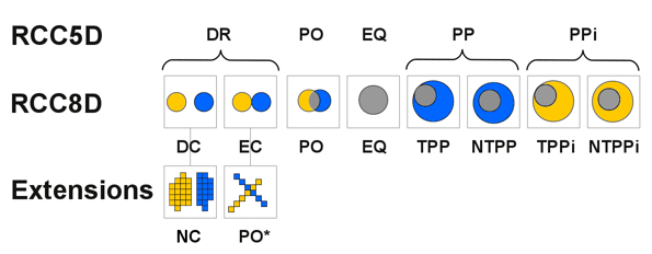
In RCC5D logic, the spatial relations between two regions are: DR (disjoint), PO (partial overlap), EQ (equal), PP (proper part) and PPi (proper part inverted).
In RCC8D logic, the spatial relations between two regions are: DC (disconnected), EC (externally connected), PO (partial overlap), EQ (equal), TPP (tangential proper part), NTPP (non-tangential proper part, TPPi (tangential proper part inverted) and NTPPi (non-tangential proper part inverted)
We have implemented some additional relations (option RCC8D+ in the plugin) such as:
- NC (neighbour connected), where two regions are separated by a one-dilation distance (that is, d <= sqrt(8) ), and
- PO* which is a case of apparent partial overlap of pixel-thin regions that cross over in particular patterns and where there are no overlapping pixels. This relation is otherwise considered EC in RCC8D or DR in RCC5D.
However, note that these new relations can and probably will change or be renamed in future versions of the plugin. Therefore it would be safer to restrict any development to the relations supported in the RCC5D and RCC8D logics.
Computing the relation between 2 regions
This example addresses the computation of the relation between two binary regions X and Y (residing in different images a.png and b.png), akin to the situation of channels in multichannel imaging such in confocal microscopy, or via colour separation with colour deconvolution. The question is: what is the relation of object X with respect to object Y?
There are some specific requirements, namely, the images containing the regions:
- must have the same size,
- the images must be aligned (so the space is represented by the same coordinates in both image, like two registered channels in a composite confocal image)
- must be 8-bit binary images
- the regions must be encoded as “white” (255) on a “black” (0) background.
 Image a.png
  Image b.png
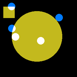
Image ab.png (below) shows more easily the overlap between the two regions:
 Image ab.png
The region overlap is encoded here for visualisation purpose in colours (X is dark yellow, Y is blue and the overlap in white). Note that region X overlaps completely with Y and therefore there are no yellow pixels). Here is a clearer example of the overlap labelling:
 Image overlap.png
To compute the relation between the regions, launch the RCC8D plugin and select image a.png for object X and image b.png for object Y.
Select the desired logic. The options are RCC5D or RCC8D (additional relations in the RCC8D+ option are not currently documented).
Check the “Details” box to see the details of the computation.
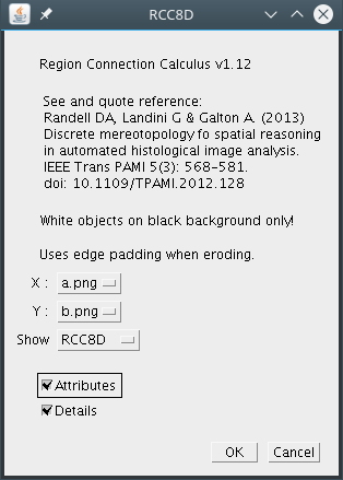
After pressing OK, a log window shows the results:
------- RCC8D -------
X: a.png
non-empty: true
b-close: true
b-open: false
regular: false
null-interior: false
border: false
atomic: false
Y: b.png
non-empty: true
b-close: true
b-open: true
regular: true
null-interior: false
border: false
atomic: false
Result : 8
NTPP
The output:
The first line gives the logic used (in this case it is RCC8D).
The next line indicates that the name of the image X (in this case it is a.png).
A list of 7 attributes of the region in image X follows:
Non-empty: is true when the region exists (i.e. there are pixels representing the region).
B-close: is true when the region remains unchanged after a morphological closing operation
B-open: is true when the region remains unchanged after a morphological opening operation
Regular: is true when the region is both B-open and B-close
Null-interior: is true when the region has no interior (i.e. region disappears after one erosion)
Border: is true if the region intersects the border of the image
Atomic: is true when the region is formed by 1 pixel
Next is the same list of attributes for region Y which exists (in this case) in image b.png.
Finally the result of the calculation is given as a numeric code “8” followed by another line showing the label, in this case “NTPP“. That is, in the example “region X is a non-tangential proper part of region Y“.
The full list of numeric codes and corresponding labels is:
Code     Label         Logic (RCC)
0         DR            5D
1         PO            5D / 8D / 8D+
2         EQ            5D / 8D / 8D+
3         PP            5D
4         PPi           5D
5         DC            8D
6         EC            8D
7         TPP           8D
8         NTPP          8D
9         TPPi          8D
10        NTPPi         8D
11        NCNTPP        8D+
12        NCNTPPi       8D+
13        NC            8D+
14        PO*           8D+
15        NTPP+         8D+
16        NTPPi+        8D+
17        DC+           8D+
18        RC+           8D+
19        DR_0          5D / 8D / 8D+
20        Unknown	5D / 8D / 8D+
DR_0 is the label of the relation (DR) returned when one or both images are empty. Relations 11, 12, 15, 16, 17 and 18 are currently undocumented and subject to change.
Example – pairs of single (i.e. connected component) regions
An example of how to apply the RCC in a macro for testing the 2 images above (a.png and b.png) in RCC8D mode:
run("RCC8D ", "x=a.png y=b.png show=RCC8D ");
Note that the results of the operation do not need to be shown in the log window, as these can be programmatically obtained via the image attributes. In this case, we use the attribute RCC to retrieve the relation label.
 selectWindow("a.png");
 myResult = call("ImpProps.getProperty", "RCC");
 print (myResult);
The code above stores the value “NTPP” in the variable myResult.
The list of supported attributes is accessed through 10 attribute keys which are set by the plugin to the images submitted after the RCC has been computed.
Key------      Possible values------
mode           RCC5D RCC8D RCC8D+
RCC            DR PO EQ PP PPi DC EC TPP NTPP TPPi NTPPi NCNTPP NCNTPPi NC PO*
               NTPP+ NTPPi+ DC+ EC+ DR_0 Unknown
RCCNum         0 1 2 3 4 5 6 7 8 9 10 11 12 13 14 15 16 17 18 19 20
non-empty      true,  false
b-close        true,  false
b-open         true,  false
regular        true,  false
null-interior  true,  false
border         true,  false
atomic         true,  false
Note that some spatial relations (PP, TPP, NTPP, NNTPP) are not symmetrical, and therefore it matters which image is queried. In the example above: NTPP(X,Y) implies NTPPi(Y,X), (note that swapping the images implies inversion of the relation), therefore the code returned is either 8 or 10 depending which image is queried.
Regions do not have to be necesarily self-connected, but they can be fragmented. Image c.png, below, contains a region that is made of 3 different clusters. The relation in this case is PO: “region X partially overlaps region Y“.
 Image c.png Image b.png
The overlap image (below) shows that only certain parts of region X (in c.png) overlap region Y (in b.png):

Where one or both regions are null, the DR relation holds. To mark this situation, the plugin returns DR_0 instead of DR (which is returned for the cases where the regions are non-null). In the case of DR_0 it is possible to know the null region(s) via the non-empty attribute key described above.
Example – pairs of fragmented regions
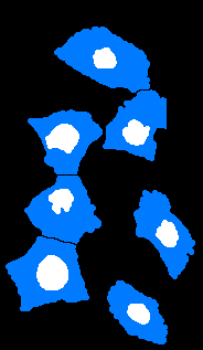
As mentioned above, regions in DM need not be restricted to connected components. Any number of regions can be summed (union) together to form a single (possibly fragmented) region. For example, image X below represents a number of nuclei (nuc.png) and image Y their cell profiles/cytoplasms (cyt.png). We can check the relation held between the set of nuclei and the set of cytplasms as single (but fragmented) regions.
This is useful for assessing in a histological context, whether nuclei and cell profiles segmented in different channels match the expected model of cells, where the nucleus is in PP(nuc,cyt) relation to the cell profile (in RCC8D this is TPP(nuc,cyt) or NTPP(nuc,cyt) ).
We test the two images below as single fragmented regions. If the RCC5D relation returned is PP(nuc,cyt) this means that nuclei are contained within the cytoplasmic regions.
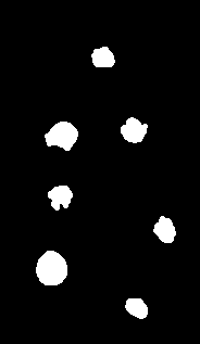 Image nuc.png
 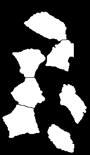 Image cyt.png
And below is the overlap image showing the relation between the (fragmented) region in nuc.png and the region in cyt.png:
The output from the plugin using RCC5D is PP(nuc,cyt):
------- RCC5D -------
X: nuc.png
non-empty: true
b-close: false
b-open: true
regular: false
null-interior: false
border: false
atomic: false
Y: cyt.png
non-empty: true
b-close: false
b-open: false
regular: false
null-interior: false
border: false
atomic: false
Result : 3
PP
When using RCC8D logic, the result is NTPP(nuc,cyt).
This shows how -in an unsupervised manner- it can be concluded that the nuc region is a proper part of the cyt region. It does not say whether all the individual nuclei are in separate cytoplasmic regions (as would be expected for a single nucleated cell model) or all in the same cyt sub-region. That is a problem needs to be resolved by comparing multiple regions (discussed below). However this result alone is useful to characterise the correctness of the segmentation results and, alternatively, if the expected model is not matched, to find out which image modification in terms of a specified minimal change (i.e. additional morphological operations) can improve the segmentation (see our IEEE-TPAMI publication for examples using conceptual neighbourhood diagrams).
Computing relations between multiple regions
In the case of multiple objects in each channel (X and Y), one way to achieve this is to extract one region at a time from the first channel (X) and compute the relations to one region at a time in the second channel (Y).
When the multiple regions we operate on are self-connected (i.e. each region is one connected piece), there are a number of shortcuts that can be exploited to speed up the process and avoid unnecessary computation: e.g. restricting the pair-wise operations to regions which are non-DR (for RCC5D mode) or non-DC (for RCC8D mode) and label DR or DC to the rest. This was implemented in the plugin named RCC8D_Multi, however we have developed a new algorithm (implemented in the RCC8D_UF_Multi plugin) with a performance improvement of over three orders of magnitude. See reference [4] for the complexity analysis of the algorithm, as well as a number of new applications of DM in mathematical morphology such as minimal opening and minimal closing.
The RCC8D_UF_Multi plugin generates a table of relationships between all the objects in the two images. The result is stored in an 8 bit image named RCC where the pixel coordinates x and y encode the regions indexes in image X and Y respectively and the pixel value value is the numerical relation code between those two regions. This means that row 0 in the image encodes the relationships between the first particle (index 0) in image X and all the particles in image Y.
Again, some image attributes are set to the RCC table and these can be accessed also via keys so the table can be queried once it has been generated:
 Key------   Values------
 mode        RCC5D RCC8D RCC8D+
 imageX      name of imageX
 imageY      name of imageY
Example – multiple regions
Here we compute the spatial relations between the connected components in images x.png and y.png.
 Image x.png
 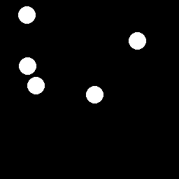 Image y.png
The overlap image (below) shows the relations between the multiple regions in x.png and y.png:
After running the plugin RCC8D_UF_Multi a table image (RCC) is generated where pixels values encode the relations between regions in the first image (x coordinate) and the regions in the other image (y coordinate) as shown next:
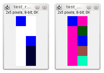 RCC5D (left) and RCC8D (right) tables (zoomed to show the individual pixels).
The RCC tables for RCC5D and RCC8D shown above are 2×5 pixels, indicating that there are two regions in image x.png and five regions in image y.png.
The colour index of pixel (0,0) the RCC5D table (left) is “1” (shown as blue; it is an 8 bit image using the Glasbey false colour look up table). This pixel encodes the relation between the index 0 region in image x.png and region index 0 in image y.png. The code “1” corresponds to the relation PO. The full list of codes with their names was given earlier, but can also be shown by clicking on the ‘Legend’ option of the plugin dialogue. That option generates the following references depending on the RCC type selected:
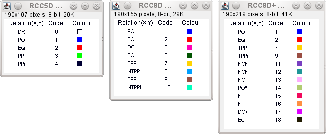
Further processing of relations data
Once the RCC table is generated, it can be used to guide further processing of regions. From the example above, we know that assuming RCC5D, region index 1 in image X is in PPi with regions indexes 3 and 4, so this information is useful to enable processing certain regions further (e.g. extraction, deletion, filtering, etc).
Here is a way to do this. The regions indexes can be obtained using ImageJ’s Particle Analyser or the Particles8 plugin included in the Morphology collection (for reference, the images can also be numerically labelled using the NumberParticles8 plugin in the same collection and facilitate localisation). To manipulate individual regions it is convenient to use the indexed XStart, YStart coordinates and the process called “binary reconstruction”. The following code extracts the starting points for all the particles in an image and stores them in the arrays x[ ] and y[ ].
run("Particles8 ", "white show=Particles minimum=0 maximum=9999999 overwrite redirect=None");
nRes=nResults;
if (nRes==0)exit("No objects in the image.");
x=newArray(nRes);
y=newArray(nRes);
//-- get the coordinates of each region in the image
for (j=0; j<nRes; j++) {
  x[j] = getResult('XStart', j);
  y[j] = getResult('YStart', j);
}
Once extracted, those coordinates can be used to select a particular region by their index: e.g. we retrieve region index 2 in image Y using reconstruction:
1. Select image Y
2. Duplicate the image (let’s call it “Seed”),
3. Set all pixels to 0 (background) and set pixel the XStart YStart pixel stored in x[2], y[2] to the foreground value (255).
4. Now use the BinaryReconstruct plugin to reconstruct the original (image Y) using the new “Seed” image as the reconstruction seed.
The result of this procedure should result in the reconstruction of only region 2 in the new image.