This section explains methods to do background illumination correction in brightfield microscopy.
Background correction can be applied while acquiring images (a priori) or after acquisition (a posteriori). The difference is that a priori correction uses images of the illumination source obtained at the time of image capture in order to characterise the illumination, while a posteriori correction assumes some ideal illumination model which might or might not be fulfilled in the already acquired images. A priori methods are, understandably, a better option.
In digital microscopy images there are several sources of image degradation:
- Camera noise
- Random noise. This is due to uncorrelated fluctuations above and below the image intensity as a consequence to the nature of the image sensors. These fluctuations vary with time (they differ from one shot to the next) and can be reduced by averaging several consecutive images or frames (assuming that the specimen does not move and that there is no vibration of the equipment). Frame averaging, however, tends to soften the image (i.e. some loss of sharpness). The magnitude of the noise reduction achieved by averaging is proportional to the square root of the number of images. This means that reducing the noise by half requires averaging 4 images; to reduce noise to one fourth requires averaging 16 images, and so on.
- Fixed pattern noise (“hot pixels”) is characterised by pixel intensities that are consistently above random noise fluctuations and it is due to faulty CCD or pixel differences in charge leakage rate (also called the “electronic bias” of the sensor). Fixed pattern noise can become apparent when using long exposure times (e.g. in fluorescence microscopy) and gets more accentuated with higher temperatures (the reason why some cameras are “cooled” to minimise this). Hot pixels appear as bright points in the image always at the same location across images. These can be compensated the by subtraction of the so-called Darkfield (a shot with the microscope camera but with light path obstructed, using the same settings as a normal shot, see below).
- Banding noise can arise during the process of reading the data from the digital sensor or by interference with other electronic equipment. This type of periodic noise can be minimised to some extent by means of Fourier filtering.
- The background illumination intensity provided by the microscope light source optics is most often not homogeneous across the field of view (microscope condensers do not always provide flat field illumination and commonly a bright spot can be detected in the middle of the image).
- The colour temperature of the light source can also affect image quality. Light sources have a characteristic radiation spectrum. In most incandescent filament lights the spectrum varies according to the temperature of the filament (i.e. the voltage applied to the lamp; with lower voltages the light becomes yellow-reddish while with higher voltages, it becomes bluish). Consequently images taken at different times may exhibit backgrounds with slightly different hues. This makes it difficult to standardise procedures such as colour segmentation, stain separation, hue quantification, etc. Some microscopes feature a switch to preset a voltage to the bulb so it delivers the same intensity and colour temperature (typically about 3200K to match indoor type B photographic film). When fixed voltages are used, then the intensity of the light is typically controlled using neutral density filters in the light path.
Acquisition (a priori) correction
1. Camera and microscope settings
- This assumes that the microscope is properly set for Köhler illumination (if you are unsure about this, there are various good tutorials and videos in the Internet).
- Consider using a light source with an infrared filter (sometimes called “heat filter”).
- Switch on all the equipment and leave it warm up for some time. The warming up time depends on room temperature, how sensitive the equipment is to temperature and how long it takes to stabilise. This can be found by taking a series of background shots over of time and plotting average intensity vs time. When the setup becomes more or less stable, the plot should show a plateau (no changes in average intensity). It is best to do image capture after reaching that plateau.
- Switch off the camera auto-gain (or auto-exposure) function. If the camera cannot switch off the auto-gain feature (like in most webcams), the method described here will not work. If you are using a standard photographic camera, set it to Manual Mode and adjust shutter speed and ISO sensitivity to achieve the best exposure setting.
- Put the specimen on the stage, focus the object, adjust the light or add/remove neutral density filters, set an appropriate camera exposure time.
- If the camera has a white balance function, apply it now on the empty illuminated bright field: remove the specimen and then apply the white balance.
- Check the histogram of this bright field to ensure it is not saturated and not too dark. If needed, re-adjust the light accordingly (or insert/remove neutral density filters) and apply white balancing again.
- Reposition the specimen and check again that the image histogram is not saturated (too many pixels at the black or white extremes) and that the grey scale values span most of the greyscale space (i.e. maximise the dynamic range). From now on, the settings of the camera and the microscope light should not be adjusted anymore.
2. Capture the Darkfield
Block the light path (do not switch the microscope light off!, most microscopes have a lever that blocks the light path to the extension tube) and capture a shot. This image will be nearly black everywhere, except for “hot pixels” if any (hot pixels might not be very noticeable but can be seen in the histogram of the image). Save the image as “Darkfield”; this will be used to compensate for hot pixels.
3. Capture the Brightfield
Now open the light path, remove the specimen (the image is all background) and capture a shot. Save it as “Brightfield”; this will be used to compensate the background illumination.
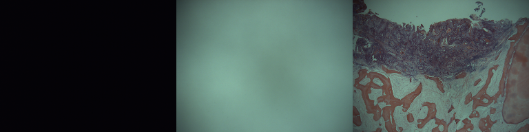
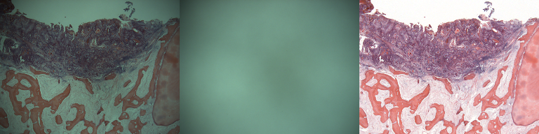
4. Capture the Specimen
Put the specimen on the stage and capture one shot. Save it as “Specimen”. Here are examples of these three shots:
5. Apply the correction
The correction operation consists of calculating the transmittance through the specimen. Transmittance is defined as the ratio of the light exiting the specimen to the light incident on the specimen. That is a value between 0 and 1, therefore to use the range of possible values stored in the image/channel, the transmittance is scaled back to the bit depth of the image minus 1 (the value of 255 in the case of 8bit channels). However the images captured to achieve this also need to be compensated for hot pixels, so the Darkfield image is subtracted before computing the transmittance according to this formula:
Corrected_Image = (Specimen - Darkfield) / (Brightfield - Darkfield) * 255
To achieve this using ImageJ, we first compensate the electronic bias (hot pixels) in the Brightfield and Specimen images. Using the command Process>ImageCalculator, calculate Brightfield – Darkfield and call the result “Divisor”:
imageCalculator("Subtract create", "Brightfield","Darkfield");
selectWindow("Result of Brightfield");
rename("Divisor");
The same is done for the Specimen image: (Specimen – Darkfield), call the result “Numerator”.
imageCalculator("Subtract create", "Specimen","Darkfield");
selectWindow("Result of Specimen");
rename("Numerator");
Next, we calculate the transmittance as the ratio of transmitted light through the specimen and the incident light to produce the corrected image. That is, the division of images: Numerator / Divisor and scale back to the 8bit range. This can achieved in a single step using the Calculator_Plus plugin which performs the division, followed by a multiplication all in double precision before pasting the clipped result back into an image:
run("Calculator Plus", "i1=Numerator i2=Divisor operation=[Divide: i2 = (i1/i2) x k1 + k2] k1=255 k2=0 create");
selectWindow("Result");
rename("Corrected");
The result of this operation should have a flat (even) background appearing white/neutral (unless the glass slide has a noticeable tint) as long as none of the settings of the camera (time, exposure, white balance etc) or the microscope settings (light, condenser, magnification) have changed between shots.
How to minimise random noise?
We can reduce random noise by taking average shots instead of single shots. In this case the Darkfield, Brightfield and Specimen images are the average of several consecutive shots. If the camera or acquiring software does not allow for average capture, it is possible to sequentially capture the images (the IJ_Robot plugin can be useful to automate this), then convert the images to a stack and finally do a Z-projection using the Average Intensity option. E.g. to average 16 shots, grab 16 images and then run:
run("Convert Images to Stack");
run("Z Project...", "start=1 stop=16 projection=[Average Intensity]");
The result is the averaged image.
What about capturing several images?
The Divisor image can be used to correct subsequent shots but only if the light source is stable and no changes are made to the microscope or camera settings. The Darkfield image can be re-used if no changes are made to the camera settings. After changing magnification (objective) or microscope light settings one can still use the same Darkfield but new Brightfield and Specimen images are required. To summarize:
- More shots in exactly the same conditions: take a new Specimen image and reuse Divisor and Darkfield.
- Changes of magnification or microscope lighting: take a new Specimen, a new Brightield image and recalculate the Divisor image (you can re-use the Darkfield).
- Changes in camera settings: take all images again.
Retrospective (a posteriori) correction
Various methods have been suggested to estimate from single images the characteristics of the background. For example:
- Fit a polynomial surface to a number of sample points (that do not contain specimen) in the image and using this as the Brightfield image for correction as above. At least 4 plugins implement this principle:
- The Shading correction (a posteriori) plugin developed at UMRS-INSERM 514 (Reims, France), here is an example.
- A plugin by Bob Dougherty is also available for fitting Legendre polynomials (Polynomial_Fit, but you have to implement subtraction of the fitted surface),
- A plugin by Michael Schmid (Fit Polynomial). This has the advantage of using the threshold to select the areas of the image to be fitted and subtract the fitted surface if desired.
- A plugin by Cory Quammen (Nonuniform Background Removal) finds a least-squares fit of background samples within the image to one of two intensity profiles: a plane, or a 2D cubic polynomial.
- Use a morphological method such as the “rolling ball” algorithm [Sternberg S. Biomedical Image Processing, IEEE Computer 1983;16(1):22-34]. This has been implemented in ImageJ as Process>Subtract Background. Be aware that this method introduces some image artefacts.
- Estimate an ‘envelope’ to the image signal as the brightfield image. [Reyes-Aldasoro CC. Retrospective shading correction algorithm based on signal envelope estimation. Electronic Letters 2009;45(9):454-456].
- Use Gaussian blurring with very large kernels and inverting the blurred image to compensate the illumination [Leong et al. Correction of uneven illumination (vignetting) in digital microscopy images. Journal of Clinical Pathology 2003;56:619-621].
- Use a minimization method to estimate the darkfield and brightfield images [Likar et al. Retrospective shading correction based on entropy minimization. Journal of Microscopy 2000;197:285-295].
However all retrospective methods make assumptions about image characteristics and illumination characteristics that might not be strictly satisfied in all cases. Most methods cannot differentiate diffuse dark regions with intense staining uptake from those with uneven background illumination. Consequently it is always preferable to correct images with an a priori method.
What about random noise?
With only one image, it is difficult to know what is noise and what is image texture. Some denoising can be achieved through image smoothing (for instance, Gaussian convolution) but this also affects edge sharpness. Median filtering preserves edges better, but still affects the image with loss of detail. Various other smoothing methods can be applied, at the expense of some loss of detail.
What about “hot pixels”?
With only one image available, one possible solution is to replace hot pixels with the average of their neighbours without affecting rest of the image.
Below is a macro that implements this idea. Note that the this version corrects single pixels, but not cluster. The pixels to filter are expected to be saturated [value=255 in 8bit greyscale images or in all channels of 24bit RGB images].
// SaturatedSinglePixelDenoising.txt
// G. Landini 16/July/2005, revised 16/July/2020
// This macro detects saturated *single* pixels (8 connected) in the
// image (grey=255) and replaces them with the pixel value of
// either the mean or the median of the neighbours (choose which
// method one by un-commenting the lines indicated below.
// Works with 8bit and 24 bit images only.
// Needs the Particles8 plugin available at:
// https://blog.bham.ac.uk/intellimic/g-landini-software/
run("Colors...", "foreground=white background=black selection=yellow");
run("Options...", "iterations=1 black count=1");
run("Duplicate...", "title=Denoised");
setBatchMode(true);
run("Duplicate...", "title=pixels");
if (bitDepth==24) run("8-bit");
setThreshold(255, 255);
run("Threshold", "thresholded remaining");

//---
// To process small clusters of pixels, rather than single pixels,
// comment the following 3 lines but be aware that the average or
// median will not be correct as other pixels in the cluster
// will also contribute to the corrected value:
run("Duplicate...", "title=non-single");
run("Particles8 ", "white show=Particles filter minimum=2 maximum=999999 overwrite");
imageCalculator("Subtract", "pixels","non-single");
close("non-single");
//---

selectWindow("Denoised");
run("Duplicate...", "title=median");

// average the 8 neighbours, comment out next line to use the median
run("Convolve...", "text1=[1 1 1 1 0 1 1 1 1] normalize");

// uncomment next line to use the median instead of the average.
// run("Median...", "radius=1");

if (bitDepth==24) {
  selectWindow("pixels");
  run("RGB Color");
}
imageCalculator("AND create", "pixels","median");
imageCalculator("Subtract", "Denoised","pixels");
imageCalculator("Add", "Denoised","Result of pixels");
setBatchMode(false);
Cite this document: Landini G. (2006-2020) Background illumination correction. Available at: https://blog.bham.ac.uk/intellimic/background-illumination-correction
Copyright © G. Landini, 2006-2020.