The two thresholding plugins discussed in this page are part of the Morphology collection.
For a detailed description of the methods, please see: Landini G, Randell DA, Fouad S, Galton A. Automatic thresholding from the gradients of region boundaries. Journal of Microscopy, 2016. (PDF)
We would be grateful if you cite the paper in any publications where you use these methods (and let us know about it).
The procedures implemented are based on a reinterpretation of the strategy observed in human operators when adjusting thresholds manually and interactively by means of ‘slider’ controls.
Users most often find the “right” threshold value by repeatedly over- and under-thresholding the image until the thresholded phase more or less coincides with the sought objects in the image.
See, for example, Russ and Russ [1]. The advantage of the computerised versions presented here is that the methods do not suffer from the uncertainty of “when to stop adjusting” the threshold.
Two different methods were implemented. The first one is a simple global thresholding procedure suitable for single or multiple global thresholds (i.e. one value for the whole image). The procedure consists of searching the greyscale space for a threshold value that generates a phase whose boundary coincides with the largest gradients in the original image. The plugin is called Threshold_Global_Gradient and it has the option of using two possible measures of the phase gradient (the mean and the total gradient).
The second method is a more interesting and complex variation of the same principle, but operates on the discrete connected components of the thresholded phase (i.e. candidate binary regions that might represent the intended object in the image) independently, therefore becoming an adaptive local thresholding procedure which operates on regions, rather than on pixels of local image subsets as is the case in the vast majority of local thresholding methods in the literature.
The procedure involves first a threshold decomposition step (where regions are extracted at all possible threshold ranges (e.g. from 0..n for dark objects). The boundaries of the binary regions thus generated are used to query the value of the average gradient at those positions in the original image. Then, the binary boundaries are labelled with that value and the ensemble of all boundaries is projected, retaining the maximum values (a maxima Z projection). The boundaries representing the highest gradients are then extracted by means of the regional maxima of the projection.
Furthermore, when combining filtering of the candidate regions based on morphological descriptors such as circularity and region size, the approach allows an efficient and clean extraction of the regions which exhibit the highest gradients.
Note that this is a computationally intensive procedure, so it is relatively slower than most other thresholding methods that process, for example, one dimensional histograms. The regional threshold plugin is called Threshold_Regional_Gradient.
Further details of the algorithms, performance and examples are included in our paper accessible through Open Access. The Java code is included in the Morphology collection.
Please note that the plugins described here use additional classes also residing in the Morphology collection, so those need to be installed, too.
Use
For ImageJ, unzip the morphology.zip file and copy the Morphology folder with all its contents the ImageJ/plugins folder restart ImageJ.
For Fiji, you can subscribe to the Mathematical Morphology update site using the Help>Update Fiji command.
After restarting ImageJ, there should be a Morphology category under the Plugins menu entry and under it are the entries for Threshold_Global_Gradient and Threshold_Regional_Gradient.
The plugins expect an 8-bit greyscale image.
Note that the Threshold_Regional_Gradient is ‘hard-wired’ to detect dark objects (low greyscale values) on a bright background (high greyscale values). To detect bright objects on a dark background, just invert the image before processing it. Please also be careful if the image is using an “inverted LUT”.
Examples
1. Global Thresholding
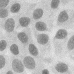
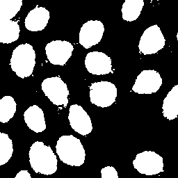
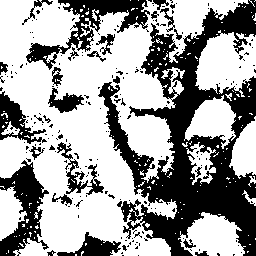
Left: original histological image of human H400 cells stained with haematoxylin. Middle: mean global gradient threshold. Right: total gradient threshold.
2. Regional Thresholding

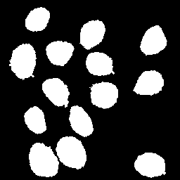
Left: maximum projection of the average gradient of the region boundaries of the image above obtained with the default plugin values (intensity in pseudocolour). Right: the morphological regional maxima was applied to extract the boundaries (in the left) with the largest gradients. These were then flood-filled. Note the clean result, devoid of any noise.
3. Regional Thresholding
The “Dot_Blot” sample image included in ImageJ provides a challenging case for segmentation. It consists of 7 x 4 dark dots of various intensities (some barely noticeable) on a grey non-uniform background. None of the 16 auto-threshold or the 9 auto-local threshold methods implemented in ImageJ can successfully extract all 28 dots cleanly. This image can be segmented by first smoothing the image with a Gaussian filter of radius=1 and then thresholding the result with the regional gradient threhsold algorithm.
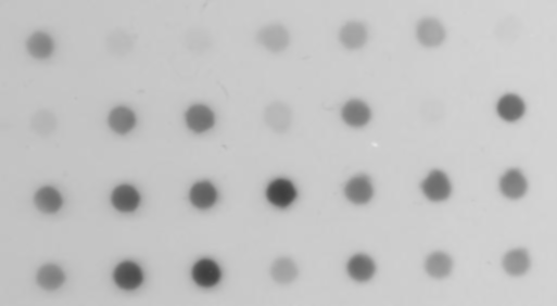
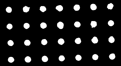
Left: original image blurred with a Gaussian filter of radius 1. Right: the result of the regional thresholding (using the default plugin values).
References
[1] Russ, J. C., Russ, C. (1987) Automatic discrimination of features in grey scale images. Journal of Microscopy 148 (3), 263-277.
[2] Landini G, Randell D, Fouad S, Galton A. Automatic thresholding from the gradients of region boundaries. Journal of Microscopy 2016, Vol 256 (2): 185-195. PDF
Acknowledgement
This work was supported by the Engineering and Physical Sciences Research Council (EPSRC), UK through funding under grant EP/M023869/1 Novel context-based segmentation algorithms for intelligent microscopy.
Back
Last updated on 7/Sep/2020