Let me introduce myself, my name is Dr Keith Evans and I’m a Physicist and Research Software Engineer. I recently started in the BEAR Research Software group as HPC software support for BlueBEAR and HPC Midlands+. On my first day, my boss gave me an objective, to run some code on the HPCs. This meant having to set up my accounts, request access; all the things a new starter needs to do. But there was another problem, I didn’t have any code to run. I needed to write some and since I like maths, pretty pictures and non-trivial parallelisation, the answer was obviously the Mandelbrot set.
For the non-mathematicians, the Mandelbrot set is the set of complex numbers (c) for which the function ![]() is not divergent.
is not divergent.
This is determined iteratively, so let’s take the example where c = 1 + 0i (c = 1):
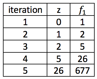
So, the complex number 1 + 0i is divergent and therefore not a member of the Mandelbrot set. To test for divergence we set a maximum magnitude of the complex number z; if z exceeds 2 then it is considered to have diverged. To complete the algorithm for determining the Mandelbrot set, we set a maximum number of iterations at which the function is considered bound. Therefore the algorithm for a determining whether a complex number belongs to the Mandlebrot set is as follows:
do while ( abs( z_complex ) .le. 2.0_rkind .and. iterations .lt. maximum_iterations )
z_complex = z_complex**2 + c_complex
iterations = iterations + 1_ikind
end do
Obviously, my algorithm is written in glorious Fortran as is 70% of all scientific software.
This algorithm returns either the number of iterations it took for the function to exceed a magnitude of 2 [ abs( z_complex ) ] or the maximum_iterations for a given complex number c. Now we can map out complex number space with orthogonal axes of the real and imaginary parts of the complex number, which we will denote as a and b, therefore the complex number c = a + bi. This will generate a 2-dimensional dataset of constant a or b from which we can plot an image using the above defined iterations variable.
We do this simply in Fortran, as multidimensional arrays are standard, but we need to define limits in the real and imaginary dimension which we will call real_lower, imaginary_lower to represent the lower limits and real_upper, imaginary_upper to represent the upper limits as well as image dimensions as image_width and image_height.
do ind = 1, image_width
do jnd = 1,image_height
c_complex = cmplx( ( ind / image_width ) * ( real_upper – real_lower ) , &
( jnd / image_height ) * ( imaginary_upper – imaginary_lower ) )
do while ( abs( z_complex ) .le. 2.0_rkind .and. iterations .lt. maximum_iterations )
z_complex = z_complex**2 + c_complex
iterations = iterations + 1_ikind
end do
mandelbrot_image( jnd , ind ) = iterations
end do
end do
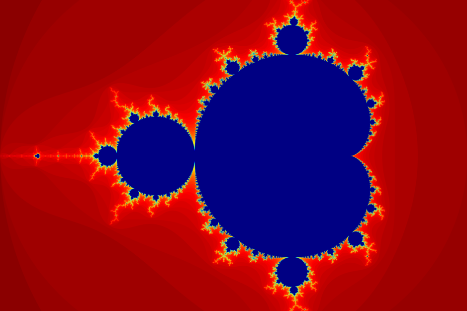
With that we have an algorithm and in fact, code to calculate the Mandelbrot set for a given range in complex space. The Mandelbrot set manifests in an attractive multi-coloured fractal pattern, this is because the algorithm above is not a yes/no, it instead returns the number of iterations it took to determine if the complex was bound or not. Strongly divergent complex values will exit quickly and return a low number (red), weakly divergent complex numbers will return a high value (blue). This results in a brightly and varied coloured image and what’s more interesting – infinitely complex – zoom in further and more detail appears, further again and more detail still and so on. So, this presents a computational problem, we want to see as much detail as possible, but double the resolution and quadruple the number of pixels. So, what happens when we want 105 pixels along each dimension? That’s 1010 pixels, if each pixel required a single calculation then 1010 operations, but they don’t, they require between 1 and maximum_iterations operations, which I set at 255.
That’s a lot of operations for a single core, in my next blog post I’ll explain how we can we parallelise such a problem to speed it up.